
Manders’ Correlation Coefficients#
# /// script
# requires-python = ">=3.12"
# dependencies = [
#     "matplotlib",
#     "ndv[jupyter,vispy]",
#     "scikit-image",
#     "numpy",
#     "scipy",
#     "tifffile",
#     "imagecodecs",
#     "tqdm",
#     "coloc_tools @ git+https://github.com/fdrgsp/coloc-tools.git"
# ]
# ///
Description#
In this notebook, we will explore how to implement Manders’ Correlation Coefficients in Python, a common method for quantifying colocalization based on pixel intensities.
The images we will use for this section can be downloaded from the Manders’ & Pearson’s Colocalization Dataset.
Note: This notebook aims to show how to practically implement these methods but does not aim to describe when to use this method. The images used have been selected to showcase the practical implementation of the methods.
Note: In this example, we will not perform any image processing steps before computing the Manders' Correlation Coefficients since the image provided has been corrected already. However, when conducting a real colocalization analysis, you should consider applying some image processing steps to clean the images before computing the Manders' Correlation Coefficients, such as background subtraction, flat-field correction, etc.
Note: In this notebook, we will only use a single image pair for demonstration purposes. Often, Manders' coefficients should not be interpreted as absolute values in isolation. Instead, it's always recommended to consider them in the context of comparisons between different conditions, controls, treatments, or experimental groups. The relative changes and ratios between conditions are often more meaningful than the absolute coefficient values themselves.
Manders’ Correlation Coefficients#
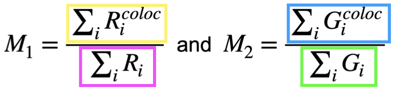
Manders’ correlation coefficients can be used to quantify the degree of colocalization between two channels (or images). These coefficients, M1 and M2, are calculated based on the pixel intensities of the two channels and for this reason, they are different from a simple area overlap.

M1 measures the fraction of channel 1 (\(R^{}\)) intensity that sits where channel 2 (\(G^{}\)) is present:
Numerator: sum of channel 1 in every pixel (\(R_i^{}\)) where
channel 2 is above the channel 2 threshold (\(G_i^{}\)), and
channel 1 is above the channel 1 threshold (\(R_i^{}\))(if you set one).
Denominator: sum of \(R_i^{}\) (channel 1) in every pixel where \(R_i^{}\) is above the \(R_i^{}\)-threshold.
M2 measures the fraction of channel 2 (\(G^{}\)) intensity that sits where channel 1 (\(R^{}\)) is present:
Numerator: sum of channel 2 in every pixel (\(G_i^{}\)) where
channel 1 (\(R_i^{}\)) is above the channel 1 threshold (\(R_i^{}\)), and
channel 2 (\(G_i^{}\)) is above the channel 2 threshold (\(G_i^{}\)) (if you set one).
Denominator: sum of channel 2 in every pixel (\(G_i^{}\)) where channel 2 (\(G_i^{}\)) is above the channel 2 threshold (\(G_i^{}\)).
For this exercise, we will analyze an image of a HeLa cell stained with two fluorescent markers: channel 1 labels endosomes and channel 2 labels lysosomes (Manders’ & Pearson’s Colocalization Dataset.)
From a biological perspective, lysosomes are typically found within or closely associated with endosomal compartments, while endosomes have a broader cellular distribution. Based on this biology, we expect:
High M2 coefficient: Most lysosomal signal should colocalize with endosomal regions
Lower M1 coefficient: Only a subset of endosomal signal should colocalize with lysosomes, since endosomes are more widely distributed throughout the cell.
Import Libraries#
import matplotlib.pyplot as plt
import ndv
import numpy as np
import tifffile
from coloc_tools import (
    manders_image_rotation_test,
    manders_image_rotation_test_plot,
    manders_image_translation_randomization,
    pca_auto_threshold,
)
from skimage.filters import threshold_otsu
Load and Visualize the Image#
Open and visualize (with ndv) the image named cells_manders_14na.tif from the Manders’ & Pearson’s Colocalization Dataset. This is a two-channel image where channel 1 has stained endosomes and channel 2 has stained lysosomes.
# Open the image
img_path = "../../_static/images/coloc/cells_manders_14na.tif"
img = tifffile.imread(img_path)
# Visualize the image
ndv.imshow(img)

To compute Manders’ Correlation Coefficients, we need two separate images (channels).
What is the image shape? How do we split the channels?
# Get image shape
print("Image shape:", img.shape)
Image shape: (2, 512, 512)
# Split the image into channels
ch1 = img[0]
ch2 = img[1]
Calculate Numerators and Denominators for Manders’ Correlation Coefficients#
The first and key step is to calculate \(R_i^{}\) and \(G_i^{}\) and thus to select which areas of each channel we want to consider for the colocalization analysis. This means we first need to threshold each images to select only the pixels we want to consider.
It is therefore evident that Manders’ Correlation Coefficients are sensitive to thresholding, the way you decide to threshold your images will have a large impact on the results.
For this example, we will first use a simple Otsu thresholding method and later in the notebook we will explore a more automated way of selecting the threshold.
# Create binary masks based on thresholds
image_1_mask = ch1 > threshold_otsu(ch1)
image_2_mask = ch2 > threshold_otsu(ch2)
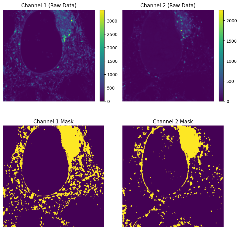
We can plot the raw data and the masks in a 2x2 subplot to visualize the results of the thresholding.
# Plot raw data and masks in a 2x2 subplot
fig, ax = plt.subplots(2, 2, figsize=(8, 8))
# Raw channel 1
im1 = ax[0, 0].imshow(ch1)
ax[0, 0].set_title("Channel 1 (Raw Data)")
ax[0, 0].axis("off")
plt.colorbar(im1, ax=ax[0, 0], fraction=0.045)
# Raw channel 2
im2 = ax[0, 1].imshow(ch2)
ax[0, 1].set_title("Channel 2 (Raw Data)")
ax[0, 1].axis("off")
plt.colorbar(im2, ax=ax[0, 1], fraction=0.045)
# Channel 1 mask
ax[1, 0].imshow(image_1_mask)
ax[1, 0].set_title("Channel 1 Mask")
ax[1, 0].axis("off")
# Channel 2 mask
ax[1, 1].imshow(image_2_mask)
ax[1, 1].set_title("Channel 2 Mask")
ax[1, 1].axis("off")
plt.tight_layout()
plt.show()
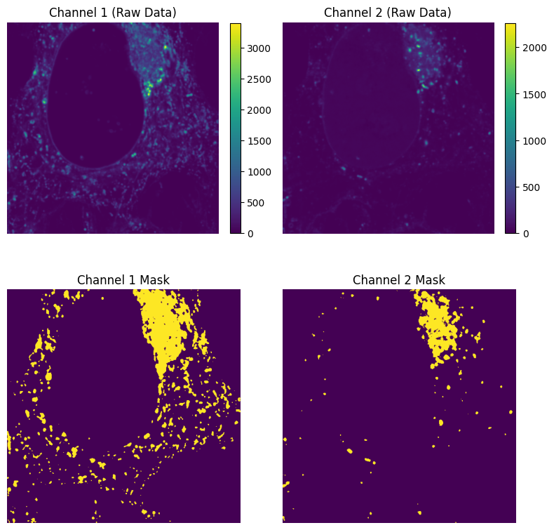
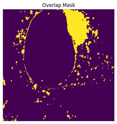
Now that we have the mask for each channel, we can first calculate the overlap mask where both channels are above their respective thresholds, and then calculate \(R_i^{coloc}\) and \(G_i^{coloc}\).
# Get the overlap mask using a logical AND operation
overlap_mask = image_1_mask & image_2_mask

# Plot overlap mask
plt.figure(figsize=(5, 5))
plt.imshow(overlap_mask)
plt.title("Overlap Mask")
plt.axis("off")
plt.show()
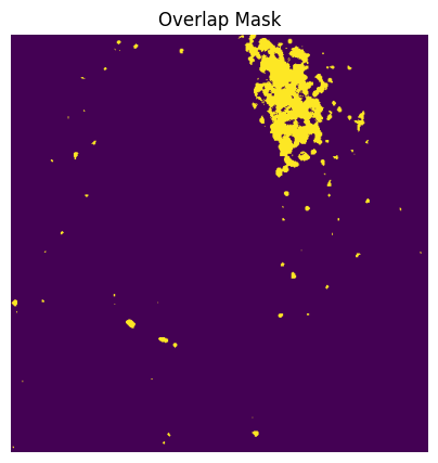
With the overlap mask, we can now calculate the \(R_i^{coloc}\) (ch1_coloc) and \(G_i^{coloc}\) (ch2_coloc) and the numerator for the Manders’ Correlation Coefficients: sum(\(R_i^{coloc}\)) and sum(\(G_i^{coloc}\)).
# Numerator
# Extract intensity from channel 1 only at pixels where both channels overlap
ch1_coloc = ch1[overlap_mask]
# Extract intensity from channel 2 only at pixels where both channels overlap
ch2_coloc = ch2[overlap_mask]

# Calculate the numerator for the Manders coefficients
m1_numerator = np.sum(ch1_coloc)
m2_numerator = np.sum(ch2_coloc)
We can now calculate the denominator for the Manders coefficients.
The denominator is the sum of the pixel intensities in the overlap mask for each channel above their respective thresholds: sum(\(R_i^{}\)) and sum(\(G_i^{}\)).
# Denominator
# Calculate the sum of the intensities in channel 1 and channel 2 above their
# respective thresholds
ch1_tr = ch1[image_1_mask]
ch2_tr = ch2[image_2_mask]
m1_denominator = np.sum(ch1_tr)
m2_denominator = np.sum(ch2_tr)
Calculate Manders’ Correlation Coefficients#
Now with both numerators and denominators calculated, we can compute the Manders coefficients M1 and M2.
# Calculate the Manders coefficients
M1 = m1_numerator / m1_denominator
M2 = m2_numerator / m2_denominator

print(f"Manders coefficient M1: {M1:.2f}")
print(f"Manders coefficient M2: {M2:.2f}")
Manders coefficient M1: 0.35
Manders coefficient M2: 0.90
With Otsu thresholding for both channels, we obtain:
M1=0.3496 and M2=0.8975
M1 indicates that approximately 35% (0.3496) of channel 1’s intensity colocalizes with channel 2. This means that about one-third of channel 1’s signal overlaps with areas where channel 2 is also present above threshold.
M2 indicates that approximately 90% (0.8975) of channel 2’s intensity colocalizes with channel 1. This suggests that nearly all of channel 2’s signal overlaps with areas where channel 1 is also present above threshold.
This asymmetry (M1 ≠ M2) is common and tells us that channel 2 is largely contained within areas where channel 1 is present, but channel 1 extends beyond the regions where channel 2 is found.
Bonus: In the Manders’ & Pearson’s Colocalization Dataset there is an image named cells_manders_0.3na.tif, the exact same image we just used nut acquired with a smaller numerical aperture (NA) of the objective lens.
What do you think will happen to the Manders’ coefficients if we use this image instead?
Costes Auto-Threshold Method#
As mentioned above, the Mender’s Correlation Coefficients are sensitive to thresholding, so the way you decide to threshold your images will have a large impact on the results.
The pca_auto_threshold function from coloc_tools implements the Costes auto-threshold method, which automatically determines optimal threshold values for both channels.
The method works by finding threshold values where pixels below these thresholds show no statistical correlation (Pearson correlation coefficient ≈ 0). This approach helps objectively separate true signal from background noise. The algorithm performs orthogonal regression (PCA) between the two channels to establish their relationship, then iteratively tests threshold pairs derived from this regression to identify the optimal separation point between signal and background.
Of course, the Costes auto-threshold method has limitations and may not work in certain scenarios, including:
Insufficient data: When there are too few non-zero pixels (< 10) in either channel
No linear relationship: When channels show non-linear, multiple population, or no correlation patterns.
Low variance: When one or both channels have uniform or near-uniform intensities
High background noise: When noise dominates the signal relationship
Limited dynamic range: Narrow intensity ranges or saturated pixels
In such cases, alternative thresholding methods (Otsu, manual, percentile-based) may be more appropriate.
We can now try to compute and print the Manders’ Correlation Coefficients using the Costes auto-threshold method.
Calculate Manders’ Coefficients with Costes Auto-Thresholds#
Calculate the Costes auto-thresholds for the two channels and print the thresholds.
# Calculate Costes auto-thresholds for the two channels
costes_thr_ch1, costes_thr_ch2, slope, intercept = pca_auto_threshold(ch1, ch2)
print(
    "Costes thresholds:\n"
    f"Channel 1 = {costes_thr_ch1}\n"
    f"Channel 2 = {costes_thr_ch2}\n"
    f"Regression Eq: y = {slope:.4f} * x + {intercept:.4f}"
)
Costes thresholds:
Channel 1 = 234.2145624551772
Channel 2 = 56.63162773616247
Regression Eq: y = 0.1913 * x + 12.8280
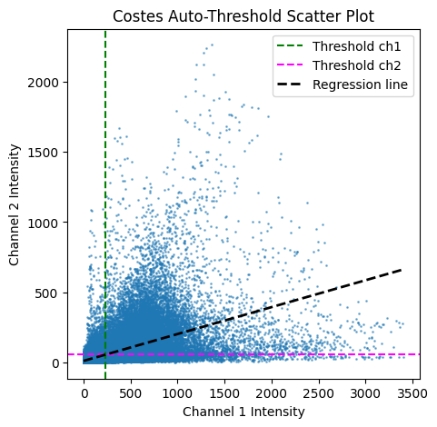
Bonus: Plot also a scatter plot of the two channels with the linear regression line.
Note that the pca_auto_threshold function returns (in order) Costes thresholds for channel 1, Costes thresholds for channel 2, slope and intercept of the linear regression. We can use the slope and intercept to plot the linear regression line.
# plot scatter plot of the two channels with thresholds
plt.figure(figsize=(5, 5))
plt.scatter(ch1.ravel(), ch2.ravel(), s=1, alpha=0.5)
plt.axvline(costes_thr_ch1, color="green", linestyle="--", label="Threshold ch1")
plt.axhline(costes_thr_ch2, color="magenta", linestyle="--", label="Threshold ch2")
x_vals = np.unique(ch1.ravel())  # Get unique intensity values from ch1
y_vals = slope * x_vals + intercept
plt.plot(
    x_vals, y_vals, color="k", linestyle="--", label="Regression line", linewidth=2
)
plt.xlabel("Channel 1 Intensity")
plt.ylabel("Channel 2 Intensity")
plt.title("Costes Auto-Threshold Scatter Plot")
plt.legend()
plt.show()
Now that we have the Costes thresholds, we can calculate the Manders’ Correlation Coefficients using the Costes thresholds as we did for the Otsu thresholds.
How do thresholds and mask images compare to the Otsu thresholds?
# Create binary masks based on thresholds
image_1_mask = ch1 > costes_thr_ch1
image_2_mask = ch2 > costes_thr_ch2

# Plot raw data and masks in a 2x2 subplot
fig, ax = plt.subplots(2, 2, figsize=(8, 8))
# Raw channel 1
im1 = ax[0, 0].imshow(ch1)
ax[0, 0].set_title("Channel 1 (Raw Data)")
ax[0, 0].axis("off")
plt.colorbar(im1, ax=ax[0, 0], fraction=0.045)
# Raw channel 2
im2 = ax[0, 1].imshow(ch2)
ax[0, 1].set_title("Channel 2 (Raw Data)")
ax[0, 1].axis("off")
plt.colorbar(im2, ax=ax[0, 1], fraction=0.045)
# Channel 1 mask
ax[1, 0].imshow(image_1_mask)
ax[1, 0].set_title("Channel 1 Mask")
ax[1, 0].axis("off")
# Channel 2 mask
ax[1, 1].imshow(image_2_mask)
ax[1, 1].set_title("Channel 2 Mask")
ax[1, 1].axis("off")
plt.tight_layout()
plt.show()
# Get the overlap mask
overlap_mask = image_1_mask & image_2_mask

# Plot overlap mask
plt.figure(figsize=(5, 5))
plt.imshow(overlap_mask)
plt.title("Overlap Mask")
plt.axis("off")
plt.show()
# Numerator
# Extract intensity from channel 1 only at pixels where both channels overlap
ch1_coloc = ch1[overlap_mask]
# Extract intensity from channel 2 only at pixels where both channels overlap
ch2_coloc = ch2[overlap_mask]

# Calculate the numerator for the Manders coefficients
m1_numerator = np.sum(ch1_coloc)
m2_numerator = np.sum(ch2_coloc)

# Denominator
# Calculate the sum of the intensities in channel 1 and channel 2 above their
# respective thresholds
ch1_tr = ch1[image_1_mask]
ch2_tr = ch2[image_2_mask]
m1_denominator = np.sum(ch1_tr)
m2_denominator = np.sum(ch2_tr)

# Calculate the Manders coefficients
M1 = m1_numerator / m1_denominator
M2 = m2_numerator / m2_denominator

print(f"Manders coefficient M1: {M1:.2f}")
print(f"Manders coefficient M2: {M2:.2f}")
Manders coefficient M1: 0.60
Manders coefficient M2: 0.84
Image Rotation Test#
The image rotation, in this context, is a statistical method to validate colocalization significance. This method applies rotations (90°, 180°, 270°) and flips (horizontal and vertical) to one channel relative to the other, then recalculates the Manders’ coefficients.
Note for Non-Square Images: When working with non-square images, rotations by 90° and 270° would change the image dimensions (e.g., a 500×512 image becomes 512×500), making direct comparison impossible. To handle this, the function automatically pads non-square images to square dimensions with zeros before applying rotations, ensuring that all transformations maintain the same image size and allow valid statistical comparisons.
The manders_image_rotation_test function provides an implementation of this method in Python. This function returns the Manders’ coefficients, the rotated/flipped Manders’ coefficients, and the p-values for both coefficients.
A low p-value (e.g. 0.0001) means that none of the rotations/flips produced M1/M2 values as high as the observed values without translation, indicating that the observed colocalization is statistically significant: the probability of getting the observed colocalization by random chance is < 0.0001 (less than 0.01%).
Let’s run it on the two channels we have been working with.
Calculate either the Otsu or Costes thresholds for the two channels and then run the image translation randomization test.
thr_1, thr_2 = threshold_otsu(ch1), threshold_otsu(ch2)
# thr_1, thr_2, _, _ = costes_auto_threshold(ch1, ch2)

# Run the rotation test
rotation_values = manders_image_rotation_test(ch1, ch2, thr_1, thr_2)
We can now print the results of the analysis: M1, M2, and their respective p-values.
# Extract results
(
    M1,
    M2,
    rot_m1_values,
    rot_m2_values,
    p_value_m1_rot,
    p_value_m2_rot,
) = rotation_values
# Print results
print(f"M1: {M1:.2f}, p-value: {p_value_m1_rot:.4f}")
print(f"M2: {M2:.2f}, p-value: {p_value_m2_rot:.4f}")
M1: 0.35, p-value: 0.0000
M2: 0.90, p-value: 0.0000
Bonus: We can also visualize the distribution of the random M1 and M2 values using a bar plot.
To do this we can simply use the manders_image_rotation_test_plot function from coloc_tools, which takes the M1 and M2 values, the rotated M1 and M2 values, and the p-values for both coefficients as input.
manders_image_rotation_test_plot(
    M1,
    M2,
    rot_m1_values,
    rot_m2_values,
    p_value_m1_rot,
    p_value_m2_rot,
)
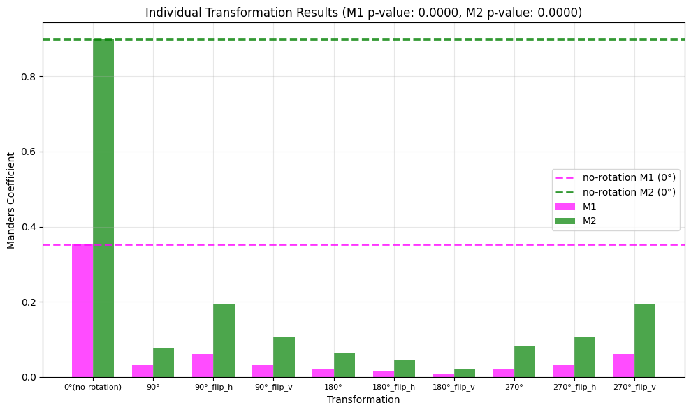
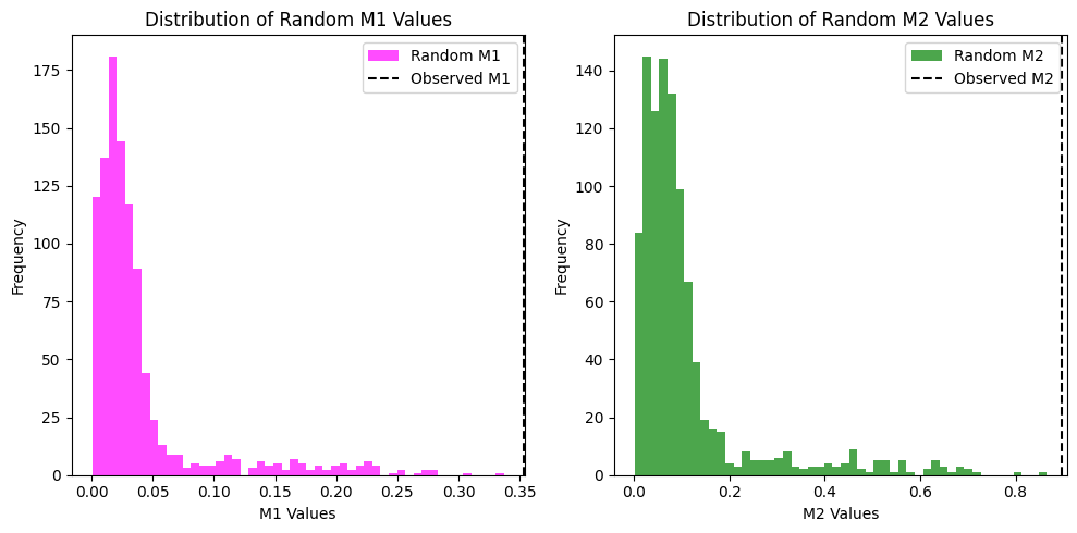
Image Translation Randomization Test#
The image translation randomization test is a statistical method used to validate the significance of colocalization results, particularly for Manders’ coefficients. This method involves randomly translating one channel relative to another and recalculating the Manders’ coefficients to create a distribution of values under the null hypothesis of no colocalization.
Note for Image Translations: Unlike rotations, translations use wraparound shifting (via np.roll()) which preserves the original image dimensions regardless of image shape. When pixels are shifted beyond the image boundaries, they wrap around to the opposite side. This ensures that all pixel intensities are preserved and no padding is required, making this method suitable for images of any dimensions.
The manders_image_translation_randomization function from coloc_tools provides an implementation of this method in Python. This function returns the Manders’ coefficients, the random Manders’ coefficients, and the p-values for both coefficients.
A low p-value (e.g. 0.0001) means that none of the n random translations (by default 1000) produced M1/M2 values as high as the observed values without translation, indicating that the observed colocalization is statistically significant: the probability of getting the observed colocalization by random chance is < 0.0001 (less than 0.01%).
Let’s run it on the two channels we have been working with.
Calculate either the Otsu or Costes thresholds for the two channels and then run the image translation randomization test.
thr_1, thr_2 = threshold_otsu(ch1), threshold_otsu(ch2)
# thr_1, thr_2, _, _ = fiji_costes_auto_threshold(ch1, ch2)

values = manders_image_translation_randomization(ch1, ch2, thr_1, thr_2)
We can now print the results of the analysis: M1, M2, and their respective p-values.
M1, M2, random_m1_values, random_m2_values, p_value_m1, p_value_m2 = values
print(f"M1: {M1:.4f}, p-value: {p_value_m1:.4f}")
print(f"M2: {M2:.4f}, p-value: {p_value_m2:.4f}")
M1: 0.3533, p-value: 0.0000
M2: 0.8981, p-value: 0.0000
Bonus: We can also visualize the distribution of the random M1 and M2 values using histograms. This will help us understand the significance of our observed values in the context of the random distributions.
# plot the distribution of random M1 and M2 values
plt.figure(figsize=(10, 5))
plt.subplot(1, 2, 1)
plt.hist(random_m1_values, bins=50, color="magenta", alpha=0.7, label="Random M1")
plt.axvline(M1, color="k", linestyle="--", label="Observed M1")
plt.xlabel("M1 Values")
plt.ylabel("Frequency")
plt.title("Distribution of Random M1 Values")
plt.legend()
plt.subplot(1, 2, 2)
plt.hist(random_m2_values, bins=50, color="green", alpha=0.7, label="Random M2")
plt.axvline(M2, color="k", linestyle="--", label="Observed M2")
plt.xlabel("M2 Values")
plt.ylabel("Frequency")
plt.title("Distribution of Random M2 Values")
plt.legend()
plt.tight_layout()
plt.show()
Summary#
The Python implementation for calculating Manders’ Correlation Coefficients is straightforward and concise, as demonstrated in the code below.
# Create binary mask for channel 1 & 2 using a thresholding method of choice
threshold_ch1, threshold_ch2 = threshold_method(ch1, ch2)
image_1_mask = ch1 > threshold_ch1
image_2_mask = ch2 > threshold_ch2

# Find pixels that are above threshold in both channels
overlap_mask = image_1_mask & image_2_mask

# Extract channel 1 & 2 intensities only from overlapping regions
ch1_coloc = ch1[overlap_mask]
ch2_coloc = ch2[overlap_mask]

# Extract all channel 1 & 2 intensities above threshold
ch1_tr = ch1[image_1_mask]
ch2_tr = ch2[image_2_mask]

# Calculate total intensity of channel 1 & 2 above threshold
sum_ch1_tr = np.sum(ch1_tr)
sum_ch2_tr = np.sum(ch2_tr)

# M1: fraction of channel 1 intensity that colocalizes with channel 2
M1 = np.sum(ch1_coloc) / sum_ch1_tr
# M2: fraction of channel 2 intensity that colocalizes with channel 1
M2 = np.sum(ch2_coloc) / sum_ch2_tr
Key Considerations for Manders’ Correlation Analysis:
Threshold Sensitivity: Manders’ coefficients are highly sensitive to thresholding methods. The choice of thresholding strategy will significantly impact your results, making careful threshold selection essential for accurate colocalization analysis. Consider using:
Automated thresholding methods (like Costes auto-threshold): these are fully automated and don’t require you to select or tune any parameters
Threshold calculation algorithms (like Otsu, Li, Triangle, Yen, etc.): these automatically calculate a threshold value, but you need to choose which algorithm to use based on your image characteristics and how the resulting threshold looks
Consistent thresholding: use the same thresholding approach across experimental conditions
Background Considerations: sometimes it is necessary to apply appropriate image preprocessing steps before calculating Manders’ coefficients such as Background subtraction to remove non-specific signal or Flat-field correction to account for illumination variations.
Statistical Validation: always validate your results using statistical tests such as the image rotation test or the image translation randomization test demonstrated above. This helps assess whether observed colocalization is statistically significant or could have occurred by chance.
Comparative Analysis: Manders’ coefficients should not be interpreted as absolute values in isolation. Instead, consider them in the context of:
Comparisons between different experimental conditions
Control vs. treatment groups
Different time points or developmental stages
Relative changes between conditions are often more meaningful than absolute values
Asymmetry Interpretation: remember that M1 ≠ M2 is common and biologically meaningful.
M1: Fraction of channel 1 intensity that overlaps with channel 2
M2: Fraction of channel 2 intensity that overlaps with channel 1
This asymmetry can reveal important biological relationships between the labeled structures