Background Correction

Download this Notebook Open in Colab

# /// script
# requires-python = ">=3.10"
# dependencies = [
#     "matplotlib",
#     "ndv[jupyter,vispy]",
#     "numpy",
#     "scikit-image",
#     "scipy",
#     "tifffile",
#     "imagecodecs",
# ]
# ///

Overview

In this notebook, we will explore different approaches to background correction in fluorescence microscopy images. Background correction is a crucial pre-processing step that helps remove unwanted background signal and improves the quality of quantitative analysis. We will use the scikit-image library to perform the background correction.

Background subtraction is useful when the background is uniform and the signal to noise ratio is high. We will demonstrate a simple background subtraction method using a sample fluorescence image. The main approaches we’ll cover are:

• Subtracting a constant background value (e.g. mode or median of the image)

• Selecting and averaging background regions to determine background level

The choice of method depends on your specific imaging conditions and the nature of the background in your images. Here we’ll demonstrate a basic approach that works well for images with relatively uniform background and distinct fluorescent signals.

Note: Background correction should be done on raw images before any other processing steps. The corrected images can then be used for further analysis like segmentation and quantification.

The images we will use for this section can be downloaded from the Measurements and Quantification Dataset.

Importing libraries

import matplotlib.pyplot as plt
import ndv
import numpy as np
import scipy
import skimage
import tifffile

Background subtraction: mode subtraction

Background subtraction can be done in different ways. If the background dominates the image as in the example we will use, the most common pixel value (the mode value) can serve as a rough background estimate to subtract from the image.

Let’s first load the image, then display it with ndv to explore the pixel values of the 07_bg_corr_nuclei.tif image.

# raw image and labeled mask
image = tifffile.imread("../../_static/images/quant/07_bg_corr_nuclei.tif")

ndv.imshow(image)

snapshot

As you can notice, most of the pixels in the image belong to the background (everything but the nuclei). Therefore, we can try to use the mode value of the image as a background estimate. We can use the scipy.stats.mode function to compute the mode of the image.

# Flatten image and get the mode
mode_val = scipy.stats.mode(image.ravel(), keepdims=False).mode
print(f"Estimated background (mode): {mode_val:.3f}")

Estimated background (mode): 33055.000

Then, we can subtract the mode value from the image and print the minimum and maximum pixel values of the resulting image.

Important: Before performing subtraction, convert the image to a floating-point (e.g., image.astype(np.float32). This prevents unsigned integer underflow, which occurs when subtracting the mode value from pixels with intensities lower than the mode. In unsigned integer formats (like uint16), negative results wrap around to very large positive values (e.g., -1 becomes 65535), leading to incorrect results.

# Subtract mode from the image (after converting to float32)
image_mode_sub = image.astype(np.float32) - mode_val
print(f"Min: {image_mode_sub.min():.2f}, Max: {image_mode_sub.max():.2f}")

Min: -71.00, Max: 3808.00

As you can see there are some negative values in the resulting image. This is because some pixels in the original image had values lower than the mode value, and when we subtract the mode from these pixels, we get negative values.

To keep working with the image, we need to handle these negative values. One common approach is to clip the negative values to zero, effectively setting any negative pixel values to zero. This is appropriate since we want background-corrected intensities to be greater than or equal to zero.

For that, we can use the numpy np.clip function to set any negative values to zero and then print the minimum and maximum pixel values of the resulting image.

image_mode_sub_to_zero = np.clip(image_mode_sub, 0, None)
print(
    f"Min: {image_mode_sub_to_zero.min():.2f}, Max: {image_mode_sub_to_zero.max():.2f}"
)

Min: 0.00, Max: 3808.00

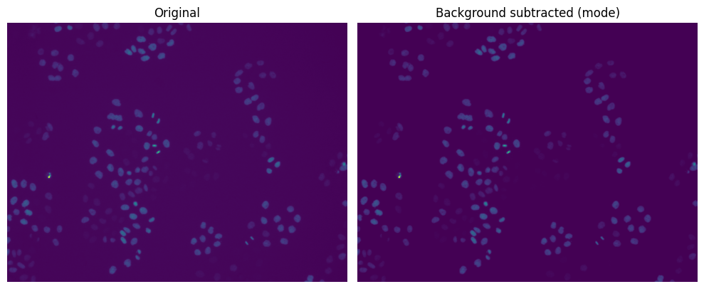
Finally, we can visualize the background-corrected image (either with matplotlib or ndv):

plt.figure(figsize=(10, 8))
plt.subplot(121)
plt.imshow(image)
plt.title("Original")
plt.axis("off")

plt.subplot(122)
plt.imshow(image_mode_sub_to_zero)
plt.title("Background subtracted (mode)")
plt.axis("off")

plt.tight_layout()
plt.show()

Background subtraction: selected regions

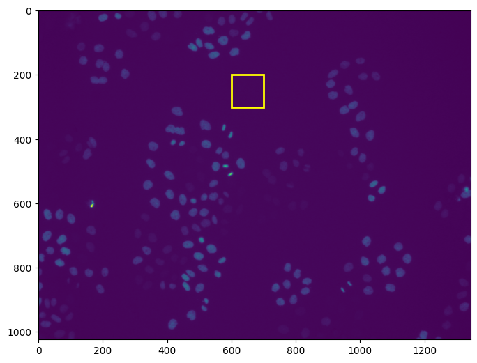
Sometimes the background isn’t uniform, or the mode isn’t representative. In these cases, we can manually choose one (or more) region we believe contains only background, estimate the average intensity in that region, and then ubtract this average value from the image.

To select regions, it might be helpful to first plot the images with the axes turned on, so we can estimate the pixel coordinates of the regions we want to select. Using matplotlib, we can even visualize and draw on the image the pixel values in the selected regions with the plt.gca().add_patch() function.

# plot the image with axis turned on to select a region
plt.figure(figsize=(8, 8))
plt.imshow(image)
# draw a rectangle around the region we want to select
x = 600
y = 200
width = 100
height = 100
plt.gca().add_patch(
    plt.Rectangle(
        (x, y),  # top-left corner
        width,  # width
        height,  # height
        edgecolor="yellow",
        facecolor="none",
        linewidth=2,
    )
)
plt.show()

Now we can calculate the mean within the selected region.

# Choose a top-left corner patch assumed to be background
# The region selected above is (600, 200) with size 100x100 therefore we can extract the
# patch as follows: [y:y+height, x:x+width]
bg_patch = image[y : y + height, x : x + width]  # image[200:300, 600:700]
bg_mean = np.mean(bg_patch)
print(f"Estimated background (mean of selected region): {bg_mean:.3f}")

Estimated background (mean of selected region): 33055.170

As we did before, we can subtract this value from the image, and clip the result to ensure no negative values remain.

image_mean_sub = image.astype(np.float32) - mode_val
print(f"Min: {image_mean_sub.min():.2f}, Max: {image_mean_sub.max():.2f}")
image_mean_sub_to_zero = np.clip(image_mean_sub, 0, None)
print(
    f"Min: {image_mean_sub_to_zero.min():.2f}, Max: {image_mean_sub_to_zero.max():.2f}"
)

Min: -71.00, Max: 3808.00
Min: 0.00, Max: 3808.00

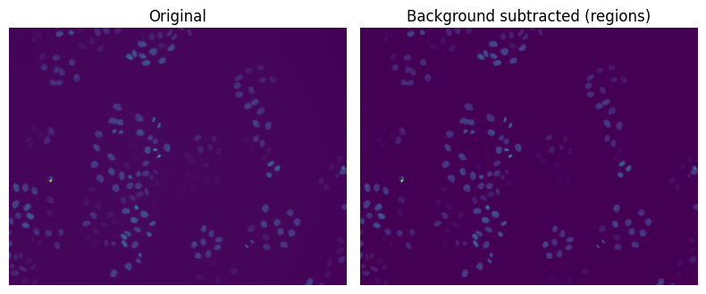
Finally, we can visualize the background-corrected image (either with matplotlib or ndv):

plt.figure(figsize=(8, 8))
plt.subplot(121)
plt.imshow(image)
plt.title("Original")
plt.axis("off")

plt.subplot(122)
plt.imshow(image_mean_sub_to_zero)
plt.title("Background subtracted (regions)")
plt.axis("off")

plt.tight_layout()
plt.show()

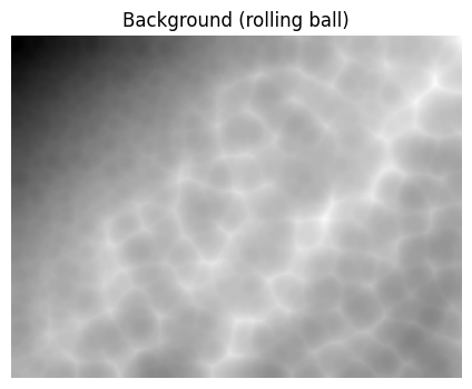
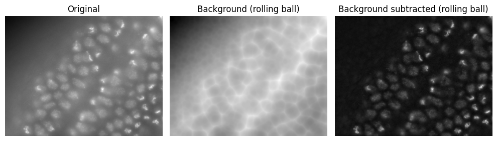
Background subtraction: rolling ball algorithm

Another way of performing background subtraction is the rolling ball algorithm. This is a method that uses a rolling ball to estimate the background. It is a good method to use when the background is not uniform.

The radius parameter configures how distant pixels should be taken into account for determining the background intensity and should be a bit bigger than the size of the structures you want to keep.

Let’s first load another image of a Drosophila embryo that has a non-uniform background:

# raw image
image = tifffile.imread("../../_static/images/quant/07_bg_corr_WF_drosophila.tif")

Let’s explore the pixel values of the image with ndv:

ndv.imshow(image)

snapshot

We can now estimate the background by using the rolling ball algorithm. Since this function returns an image (which is the background we want to subtract), we can also visualize it with matplotlib:

background_residue = skimage.restoration.rolling_ball(image, radius=100)

plt.figure(figsize=(8, 4))
plt.imshow(background_residue, cmap="gray")
plt.title("Background (rolling ball)")
plt.axis("off")
plt.show()

We can now subtract the background residue from the image and plot with matplotlib the raw image, the background image, and the background-corrected image:

image_rb_sub = image - background_residue

plt.figure(figsize=(10, 10))

plt.subplot(131)
plt.imshow(image, cmap="gray")
plt.title("Original")
plt.axis("off")

plt.subplot(132)
plt.imshow(background_residue, cmap="gray")
plt.title("Background (rolling ball)")
plt.axis("off")

plt.subplot(133)
plt.imshow(image_rb_sub, cmap="gray")
plt.title("Background subtracted (rolling ball)")
plt.axis("off")

plt.tight_layout()
plt.show()

Other Background Correction Techniques

These are more advanced or specialized techniques you can explore:

• Morphological opening: Removes small foreground objects to approximate the background.

• Gaussian/median filtering: Smooths out the image to isolate large-scale variations.

• Polynomial surface fitting: Useful when background varies gradually across the field.

• Tiled/local background subtraction: Estimate and subtract background patch-by-patch.

Your method choice should depend on image modality, signal-to-noise, and application.

A good reference for background correction is the scikit-image documentation.