
Measurements & Quantification Notebook#
# /// script
# requires-python = ">=3.10"
# dependencies = [
#     "matplotlib",
#     "numpy",
#     "scikit-image",
#     "scipy",
#     "tifffile",
#     "imagecodecs",
#     "pandas",
# ]
# ///
Overview#
In this notebook, we will explore one possible approach to extracting, measuring, and quantifying information from fluorescence microscopy images, or, in other words, how to go from images to numbers to plots.
Fluorescence images can contain a wide range of information. In this notebook, as an example, we will focus on extracting quantitative information from the fluorescence intensity and the morphology of the objects in the image, mainly using the scikit-image library.
In addition, we will learn how to save the extracted information as a .csv file using the pandas library.
The images we will use for this section can be downloaded from the Classic Segmentation Dataset. We will also need the labeled images that we created in the Classic Segmentation section.
Note: The images from the Classic Segmentation Dataset have been pre-processed to remove the background and correct for illumination variations (flat-field correction) and are therefore of type float32.
TODO: UPDATE THE LINK TO THE DATASET AND TO THE CLASSIC SEGMENTATION
Importing libraries#
from pathlib import Path

import matplotlib.pyplot as plt
import numpy as np
import pandas as pd
import skimage
import tifffile
Load and Display Images#
Let’s load and display our raw and segmented images (labeled images) with matplotlib:
image = tifffile.imread("../../_static/images/quant/DAPI_wf_10.tif")
labeled_mask = tifffile.imread("../../_static/images/quant/DAPI_wf_10_labels.tif")

# Display results
fig, axis = plt.subplots(1, 2, figsize=(8, 4))
axis[0].imshow(image, cmap="gray")
axis[0].set_title("Original")
axis[0].axis("off")
axis[1].imshow(labeled_mask, cmap="nipy_spectral")
axis[1].set_title("Labeled Mask")
axis[1].axis("off")

plt.tight_layout()
plt.show()
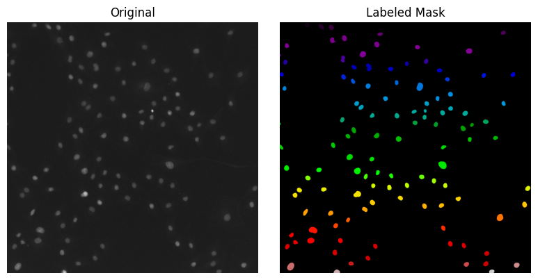
Accessing single objects in the labeled image#
Remember, a labeled image is an image where each pixel is assigned a unique value (or label) that corresponds to a specific object or region in the image, in our case, nuclei. This means that each nucleus in the image is represented by a unique value, and all pixels that belong to the same nucleus share the same value.
For example, let’s try to create a new image that contains only the pixels of the first nucleus in the labeled image:
# create an image that contains only the pixels of the first nucleus in the labeled image
nucleus_1 = labeled_mask == 1

# Plot the extracted nucleus image
plt.figure(figsize=(6, 6))
plt.imshow(nucleus_1, cmap="gray")
plt.title("Nucleus 1")
plt.axis("off")
plt.show()
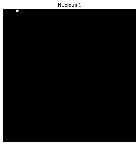
This new image we obtained is a boolean binary mask with value False for background and True for the nucleus number 1.
To verify that this is indeed a binary mask, we can query for the minimum and maximum value using the np.min() and np.max() functions:
print(np.min(nucleus_1))
print(np.max(nucleus_1))
False
True
Manual Extraction of Properties#
Now we can use this mask to extract and print the intensity values of the pixels that belong to this nucleus from the original image.
# Extract the intensity values of the pixels that belong to this nucleus from the original image
nucleus_1_intensity = image[nucleus_1]
# Print the intensity values
print(nucleus_1_intensity)
[0.14724375 0.16933577 0.20225072 ... 0.14086601 0.09265734 0.16034997]
We can then calculate and print the mean intensity using the np.mean() function:
nucleus_1_mean_intensity = np.mean(nucleus_1_intensity)
print(f"Mean intensity of nucleus 1: {nucleus_1_mean_intensity}")
Mean intensity of nucleus 1: 0.2542710304260254
Or we can measure and print the area, in pixels, of the nucleus 1. The result corresponds to the total number of pixels that have the value True in the binary mask. We can do this by using the np.sum() function:
nucleus_1_area = np.sum(nucleus_1)
print(f"Area of nucleus 1: {nucleus_1_area}")
Area of nucleus 1: 1312
To convert the area to a more meaningful unit, such as micrometers squared, we need to know the pixel size of the image.
If we assume a pixel size of 0.325 micrometers, we can convert the area from pixels to square micrometers by multiplying by the square of the pixel size:
pixel_size = 0.325  # µm
nucleus_1_area_um2 = nucleus_1_area * (pixel_size**2)
print(f"Area of nucleus 1: {nucleus_1_area_um2} um^2")
Area of nucleus 1: 138.58 um^2
Automated Extraction of Properties#
We could implement a function that would automate the extraction of intensity values or area for all nuclei in the labeled image, as well as implement more complex measurements. However, luckily, we don’t have to do it ourselves, as there are libraries that can help us with this task and more in a very efficient way.
The skimage.measure module from the scikit-image package provides several tools to measure properties of image regions. It is especially powerful when working with labeled segmentation masks, where each object in an image is assigned a unique integer label.
This module is a foundational tool for extracting morphological and intensity-based features from binary or labeled images.
A useful function in skimage.measure is regionprops:
Parameters:
label_image— A 2D or 3D array where each unique non-zero number corresponds to a labeled object (typically fromskimage.measure.label).intensity_image(optional) — The raw grayscale image associated with the label mask, used to compute intensity features like mean or standard deviation.
For example:
skimage.measure.regionprops(label_image, image)
Returns:
A
listofRegionPropertiesobjects — one for each labeled object. Each object contains attributes describing shape, position, and optionally intensity and can be accessed with dot notation (e.g.,RegionProperties.areaorRegionProperties.mean_intensity).
In the table below, we summarize some of the common features that can be extracted using this function:
Measurement |
Description |
|---|---|
area |
Measures the number of pixels in the object (size) |
perimeter |
Approximates the length around the object |
eccentricity |
Quantifies elongation—how stretched the shape is |
solidity |
Indicates shape irregularity by comparing area to convex area |
extent |
Compares object area to its bounding box area |
orientation |
Measures the angle of the major axis of the object |
mean_intensity |
Averages pixel values inside the region (if intensity image is given) |
max_intensity |
Finds the brightest pixel value inside the object |
intensity_image |
Extracts the raw intensity image cropped to the object |
centroid |
Finds the object’s center of mass (position in the image) |
bbox |
Gives the bounding box coordinates of the object |
Let’s create a variable named props to store the result of the skimage.measure.regionprops function using the labeled_mask and the original image as inputs:
props = skimage.measure.regionprops(labeled_mask, image)
Since the props variable is a list of RegionProperties, we can access the properties of each object using indexing. For example, to access the properties of the first object (or the first nucleus), we can use props[0].
props[0]
<skimage.measure._regionprops.RegionProperties at 0x7f881d356390>
From the regionprops documentation (and as mentioned above), we can see that we can access a lot of properties for each RegionProperties in the list. For example, to get the mean intensity of the first region (nucleus), we can use props[0].mean_intensity:
props[0].mean_intensity
np.float32(0.25427103)
As you can see, this answer is the same value we obtained manually before.
Note: To see all of the available properties for RegionProperties use the dir() function which will list all the attributes and methods of the object: dir(props[0]). Ignore all the methods that start with __ (double underscore) as they are special methods in Python.
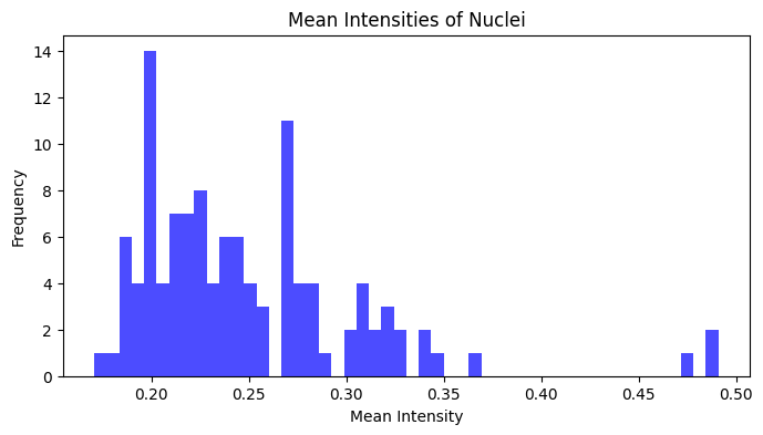
Let’s now extract the mean intensity of all nuclei and plot it using matplotlib in a histogram:
# Extract mean intensity of all regions
mean_intensities = []
for prop in props:
    mean_intensities.append(prop.mean_intensity)
# NOTE: this for loop can also be written as a list comprehension:
# mean_intensities = [prop.mean_intensity for prop in props]

# plot the mean intensities in a histogram
plt.figure(figsize=(8, 4))
plt.hist(mean_intensities, bins=50, color="blue", alpha=0.7)
plt.title("Mean Intensities of Nuclei")
plt.xlabel("Mean Intensity")
plt.ylabel("Frequency")
plt.show()
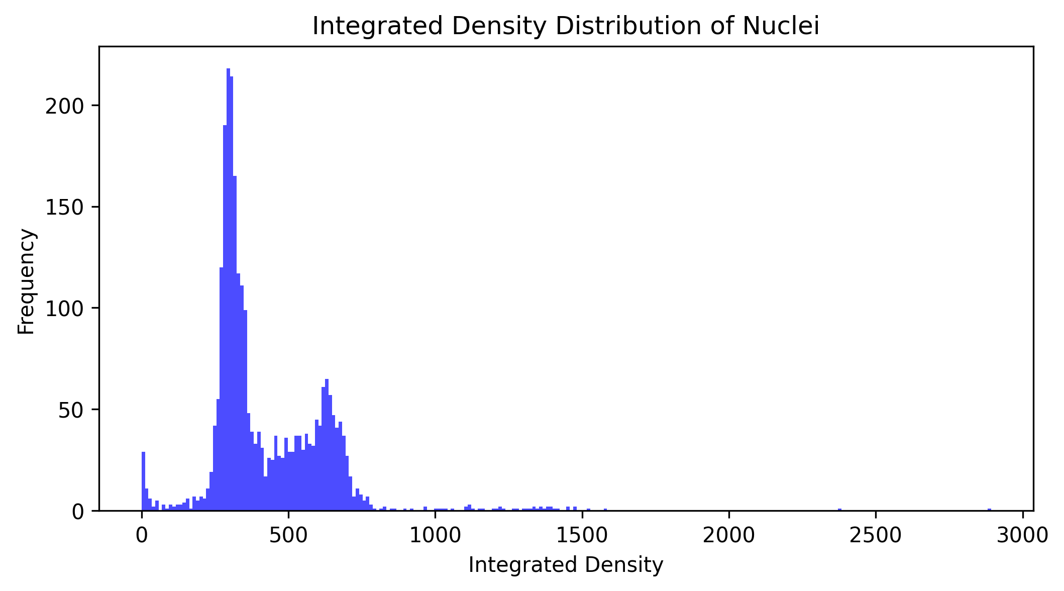
Recall that the dataset from the Classic Segmentation section contains images of HeLa cells stained with DAPI, a fluorescent dye that binds to DNA.
We know that:
Cells in the G1 phase of the cell cycle are diploid and thus have two sets of chromosomes (2n).
Cells in the G2 phase and are tetraploid (4n).
During S phase (DNA doubling), cells have a DNA content ranging between 2n and 4n.
Therefore, by looking at the DNA content (2n vs 4n) in a cell nucleus, it should be possible to discriminate between the cell cycle phases.
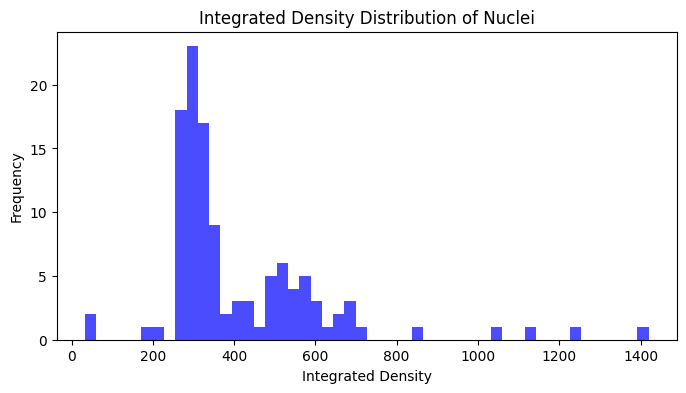
The amount of DAPI fluorescence is proportional to DNA content, so we can measure the total DAPI nuclear intensity (integrated density) to estimate the DNA content of cells. We can use these measurements to plot the cell cycle phase distribution of the entire population of cells in the dataset.
The total intensity, also known as integrated density, is defined as the sum of the pixel intensities within a region of interest, which in our case is the nucleus. To calculate it we can use the image_intensity attribute of the RegionProperties object, which contains the values of all the pixels in the region of interest (the nucleus) and sum them up using the np.sum() function.
For example:
np.sum(props[0].image_intensity)
np.float32(333.60358)
✍️ Exercise: Plot DAPI Nuclear Integrated Density Distribution from the Entire Dataset#
In this exercise, let’s do the following:
Create a
dataset_integrated_density_listlist variableWrite a
for loopthat will iterate over loading all pairs of images (raw and labeled) in the dataset to…Extract the total integrated density of each nucleus in each image
Store the results in a list named
dataset_integrated_density_list
Plot the distribution of the integrated density values using
matplotliband a histogram (bin size of 250)
raw_image_path = Path("/Users/raw_images_folder")
labels_image_path = Path("/Users/labels_images_folder")

labels_image_suffix = "_labeled.tif"  # How does the labeled image file name end?

# Create a list to store the integrated density values for all nuclei in the dataset
integrated_density_list = []

for raw_image_file in raw_image_path.glob("*.tif"):
    # Load the raw image
    raw_image = tifffile.imread(raw_image_file)
    # Get image name without extension
    image_name = raw_image_file.stem
    # Load the corresponding labeled image
    labels_image_file = labels_image_path / f"{image_name}_{labels_image_suffix}"
    if not labels_image_file.exists():
        print(f"Labels file for {image_name} not found. Skipping...")
        continue
    labeled_mask = tifffile.imread(labels_image_file)
    # Get region properties
    props = skimage.measure.regionprops(labeled_mask, intensity_image=raw_image)
    # Calculate total integrated density for each nucleus
    for prop in props:
        integrated_density = np.sum(prop.image_intensity)
        integrated_density_list.append(integrated_density)
    # same as:
    # integrated_density_list.extend([np.sum(prop.image_intensity) for prop in props])

# Plot the distribution of integrated density values
plt.figure(figsize=(8, 4))
plt.hist(integrated_density_list, bins=250, color="blue", alpha=0.7)
plt.title("Integrated Density Distribution of Nuclei")
plt.xlabel("Integrated Density")
plt.ylabel("Frequency")
plt.show()
From Properties to Tables#
There is another useful function in the skimage.measure module called regionprops_table that allows us to create a table of properties for each region in the labeled image.
Looking at the documentation, we can see that this function, returns a dict object (dictionary type as we’ve seen in Data Structures: Dictionaries) where each property is a key and the values are arrays containing the property values for each region in the labeled image.
The main attributes of this function are:
label_image: The labeled image where each unique integer corresponds to a labeled object.
intensity_image (optional): The raw grayscale image associated with the label mask (used to compute intensity features).
properties (optional): A list of properties to include in the table. If not specified, all properties will be included.
For example:
props_dict = regionprops_table(label_image, raw_image, properties=['area', 'perimeter'])
Let’s see how we can use this in practice and create a DataFrame with the image_intensity and area properties for each nucleus in the labeled image.
First we need to reload one raw image and the corresponding labeled image:
# raw image and labeled mask
image = tifffile.imread("../../_static/images/quant/DAPI_wf_10.tif")
labeled_mask = tifffile.imread("../../_static/images/quant/DAPI_wf_10_labels.tif")
Create the dictionary with the regionprops_table function that includes the label, image_intensity, and area properties, and print the keys (remember this is a dict) of the results:
props_dict = skimage.measure.regionprops_table(
    labeled_mask, intensity_image=image, properties=["label", "image_intensity", "area"]
)
print(props_dict.keys())
dict_keys(['label', 'image_intensity', 'area'])
Since props_dict is a dictionary, we can access the properties of each region using the keys of the dictionary. Each key corresponds to a property, and the associated value is an array containing the property values for each region.
For example, to access the area of each region, we can do:
areas = props_dict['area']
Similarly, we can access and print the image_intensity property (print only the first three values):
integrated_density_list = props_dict["image_intensity"]
# let's print the first three values since the list can be long
print(integrated_density_list[:3])
[array([[-0.,  0.,  0., ...,  0.,  0.,  0.],
        [ 0.,  0.,  0., ...,  0.,  0.,  0.],
        [ 0.,  0.,  0., ...,  0.,  0.,  0.],
        ...,
        [ 0.,  0.,  0., ...,  0.,  0.,  0.],
        [ 0.,  0.,  0., ...,  0.,  0.,  0.],
        [ 0.,  0.,  0., ...,  0.,  0.,  0.]], shape=(38, 45), dtype=float32)
 array([[ 0.,  0.,  0., ...,  0.,  0.,  0.],
        [ 0.,  0.,  0., ...,  0., -0.,  0.],
        [ 0.,  0.,  0., ...,  0.,  0.,  0.],
        ...,
        [ 0.,  0.,  0., ...,  0.,  0.,  0.],
        [ 0.,  0.,  0., ...,  0.,  0.,  0.],
        [ 0.,  0.,  0., ...,  0.,  0.,  0.]], shape=(51, 52), dtype=float32)
 array([[ 0.,  0.,  0., ...,  0.,  0., -0.],
        [ 0.,  0.,  0., ...,  0.,  0.,  0.],
        [ 0.,  0.,  0., ...,  0.,  0.,  0.],
        ...,
        [ 0.,  0.,  0., ...,  0.,  0.,  0.],
        [ 0.,  0.,  0., ...,  0.,  0.,  0.],
        [ 0.,  0.,  0., ...,  0., -0.,  0.]], shape=(50, 46), dtype=float32)]
While the advantage of using regionprops_table over regionprops may not be clear at this point, this regionprops_table method becomes useful when we want to create a table with all of the properties of each region in the labeled image as well as save it as a .csv file. In fact, this props_dict output can be used to directly create a **pandas** DataFrame.
pandas is a powerful Python library for data manipulation and analysis. It provides high-performance, easy-to-use data structures and tools for working with structured data. The main data structure in pandas is the DataFrame, which is a 2-dimensional labeled data structure with columns of potentially different types (like numbers, strings, arrays, etc.).
Let’s now create a DataFrame with the props_dict variable and print it:
props_df = pd.DataFrame(props_dict)
print(props_df)
     label                                    image_intensity    area
0        1  [[-0.0, 0.0, 0.0, 0.0, 0.0, -0.0, 0.0, 0.0, 0....  1312.0
1        2  [[0.0, 0.0, 0.0, 0.0, 0.0, 0.0, 0.0, 0.0, 0.0,...  1748.0
2        3  [[0.0, 0.0, 0.0, 0.0, 0.0, 0.0, 0.0, 0.0, 0.0,...  1729.0
3        4  [[0.0, 0.0, 0.0, 0.0, 0.0, 0.0, 0.0, 0.0, 0.0,...  1351.0
4        5  [[0.0, 0.0, 0.0, 0.0, 0.0, 0.0, 0.0, 0.0, 0.0,...  1185.0
..     ...                                                ...     ...
110    111  [[0.0, 0.0, 0.0, 0.0, 0.0, 0.0, 0.0, 0.0, 0.0,...  1622.0
111    112  [[0.0, 0.0, 0.0, 0.0, 0.0, 0.0, 0.0, 0.0, 0.0,...  3556.0
112    113  [[0.0, 0.0, 0.0, -0.0, 0.0, 0.0, 0.0, 0.0, 0.0...  1971.0
113    114  [[0.0, 0.0, 0.0, 0.0, 0.0, 0.0, 0.0, 0.0, 0.0,...  1488.0
114    115  [[0.0, 0.0, 0.0, 0.0, 0.0, 0.0, 0.0, 0.0, 0.0,...  1339.0

[115 rows x 3 columns]
Notice that now we have converted the dict file in a more tabular format, which is easier to work with for data analysis and manipulation tasks. The rows of the DataFrame correspond to the regions (nuclei) in the labeled image, and the columns correspond to the properties of each region.
For example, we can now access the image_intensity property by the column name as key:
image_intensity = props_df["image_intensity"]
print(image_intensity)
0      [[-0.0, 0.0, 0.0, 0.0, 0.0, -0.0, 0.0, 0.0, 0....
1      [[0.0, 0.0, 0.0, 0.0, 0.0, 0.0, 0.0, 0.0, 0.0,...
2      [[0.0, 0.0, 0.0, 0.0, 0.0, 0.0, 0.0, 0.0, 0.0,...
3      [[0.0, 0.0, 0.0, 0.0, 0.0, 0.0, 0.0, 0.0, 0.0,...
4      [[0.0, 0.0, 0.0, 0.0, 0.0, 0.0, 0.0, 0.0, 0.0,...
                             ...
110    [[0.0, 0.0, 0.0, 0.0, 0.0, 0.0, 0.0, 0.0, 0.0,...
111    [[0.0, 0.0, 0.0, 0.0, 0.0, 0.0, 0.0, 0.0, 0.0,...
112    [[0.0, 0.0, 0.0, -0.0, 0.0, 0.0, 0.0, 0.0, 0.0...
113    [[0.0, 0.0, 0.0, 0.0, 0.0, 0.0, 0.0, 0.0, 0.0,...
114    [[0.0, 0.0, 0.0, 0.0, 0.0, 0.0, 0.0, 0.0, 0.0,...
Name: image_intensity, Length: 115, dtype: object
And if we want to get the integrated density values for the first nucleus, we can do the following:
integrated_density_0 = np.sum(image_intensity[0])
print(integrated_density_0)
333.60358
To get the integrated density values for all nuclei, we can create a list where we sum the pixel intensities for each nucleus:
# Calculate integrated density for each nucleus
integrated_densities = []
for intensity_array in props_df["image_intensity"]:
    integrated_density = np.sum(intensity_array)
    integrated_densities.append(integrated_density)
# same as:
# integrated_densities = [np.sum(intensity_array) for intensity_array in props_df['image_intensity']]

# Plot histogram of integrated densities
plt.figure(figsize=(8, 4))
plt.hist(integrated_densities, bins=50, color="blue", alpha=0.7)
plt.title("Integrated Density Distribution of Nuclei")
plt.xlabel("Integrated Density")
plt.ylabel("Frequency")
plt.show()
Manipulating tables as dataframes#
Now that we have converted the measurements table into a DataFrame, we can start manipulating it.
For example, we can create a new column in the DataFrame with the integrated density per nucleus, and then display the first few rows of the DataFrame using the head() method:
# Add integrated density as a new column
props_df["integrated_density"] = integrated_densities

# Print the first few rows of the DataFrame to verify the new column
props_df.head()
| label | image_intensity | area | integrated_density | |
|---|---|---|---|---|
| 0 | 1 | [[-0.0, 0.0, 0.0, 0.0, 0.0, -0.0, 0.0, 0.0, 0.... | 1312.0 | 333.603577 |
| 1 | 2 | [[0.0, 0.0, 0.0, 0.0, 0.0, 0.0, 0.0, 0.0, 0.0,... | 1748.0 | 479.227600 |
| 2 | 3 | [[0.0, 0.0, 0.0, 0.0, 0.0, 0.0, 0.0, 0.0, 0.0,... | 1729.0 | 493.648102 |
| 3 | 4 | [[0.0, 0.0, 0.0, 0.0, 0.0, 0.0, 0.0, 0.0, 0.0,... | 1351.0 | 278.010895 |
| 4 | 5 | [[0.0, 0.0, 0.0, 0.0, 0.0, 0.0, 0.0, 0.0, 0.0,... | 1185.0 | 283.689819 |
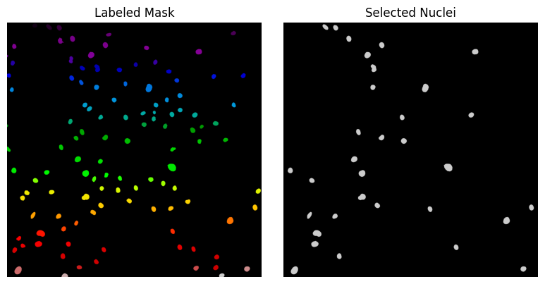
Dataframe makes conditional filtering and selection easy. We can use the loc[...] method to select rows and columns by their labels.
For example, let’s identify the percentage of nuclei that are larger than average and have high integrated density:
mean_area = props_df["area"].mean()
mean_density = props_df["integrated_density"].mean()

# conditional filtering
large_bright_nuclei = props_df.loc[
    (props_df["area"] > mean_area) & (props_df["integrated_density"] > mean_density)
]

print(
    f"% of nuclei larger than average and brighter than average: {len(large_bright_nuclei) / len(props_df) * 100}%"
)
% of nuclei larger than average and brighter than average: 27.82608695652174%
Using the np.isin(against, for) function, we can extract the labels of large and bright nuclei from the DataFrame to create a binary mask showing only those selected nuclei in the original image.
selected_labels = large_bright_nuclei["label"].values
selected_mask = np.isin(labeled_mask, selected_labels)
Once the nuclei of interest have been selected in the dataframe, it is possible to visualize them in the labeled image.
fig, axis = plt.subplots(1, 2, figsize=(8, 4))
axis[0].imshow(labeled_mask, cmap="nipy_spectral")
axis[0].set_title("Labeled Mask")
axis[0].axis("off")
axis[1].imshow(selected_mask, cmap="nipy_spectral")
axis[1].set_title("Selected Nuclei")
axis[1].axis("off")
plt.tight_layout()
plt.show()
It is also possible to select by position using .iloc[...].
For example, to select the first 10 rows of the DataFrame, we can write:
props_df.iloc[:10].head()
| label | image_intensity | area | integrated_density | |
|---|---|---|---|---|
| 0 | 1 | [[-0.0, 0.0, 0.0, 0.0, 0.0, -0.0, 0.0, 0.0, 0.... | 1312.0 | 333.603577 |
| 1 | 2 | [[0.0, 0.0, 0.0, 0.0, 0.0, 0.0, 0.0, 0.0, 0.0,... | 1748.0 | 479.227600 |
| 2 | 3 | [[0.0, 0.0, 0.0, 0.0, 0.0, 0.0, 0.0, 0.0, 0.0,... | 1729.0 | 493.648102 |
| 3 | 4 | [[0.0, 0.0, 0.0, 0.0, 0.0, 0.0, 0.0, 0.0, 0.0,... | 1351.0 | 278.010895 |
| 4 | 5 | [[0.0, 0.0, 0.0, 0.0, 0.0, 0.0, 0.0, 0.0, 0.0,... | 1185.0 | 283.689819 |
To select the first 10 rows and the first 3 columns, we can write:
props_df.iloc[:10, :3].head()
| label | image_intensity | area | |
|---|---|---|---|
| 0 | 1 | [[-0.0, 0.0, 0.0, 0.0, 0.0, -0.0, 0.0, 0.0, 0.... | 1312.0 |
| 1 | 2 | [[0.0, 0.0, 0.0, 0.0, 0.0, 0.0, 0.0, 0.0, 0.0,... | 1748.0 |
| 2 | 3 | [[0.0, 0.0, 0.0, 0.0, 0.0, 0.0, 0.0, 0.0, 0.0,... | 1729.0 |
| 3 | 4 | [[0.0, 0.0, 0.0, 0.0, 0.0, 0.0, 0.0, 0.0, 0.0,... | 1351.0 |
| 4 | 5 | [[0.0, 0.0, 0.0, 0.0, 0.0, 0.0, 0.0, 0.0, 0.0,... | 1185.0 |
Saving dataframes to CSV#
One of the most useful features of pandas is the ability to easily save data to various file formats. Let’s save our measurements to a CSV file that can be opened in spreadsheet software like Excel:
props_df.to_csv("nucleus_measurements.csv", index=False)
We can also do the reverse: use pandas to load CSV files into a pandas DataFrame with read_csv:
props_df_loaded = pd.read_csv("nucleus_measurements.csv")
# check the data
props_df_loaded.head()