Cellpose in Python#
# /// script
# requires-python = ">=3.12"
# dependencies = [
#     "matplotlib",
#     "tifffile",
#     "cellpose"
# ]
# ///
Overview#
In this section, we’ll learn how to use Cellpose, a powerful deep learning tool for cell segmentation. Cellpose works on a wide variety of microscopy images—including both nuclei and full cells—and doesn’t require retraining for many common use cases.
We’ll start by running Cellpose on a single image and then move to batch processing and visualization. Later, we’ll explore how to customize parameters and interpret Cellpose outputs like masks and flow fields.
💡 Tip: If you’re not using a GPU (or are on a Mac with Apple Silicon), we recommend running this notebook on Google Colab for faster performance.
Import Libraries#
from pathlib import Path

import matplotlib.pyplot as plt
import tifffile
from cellpose import core, io, models, plot
from tqdm import tqdm
Welcome to CellposeSAM, cellpose v
cellpose version: 	4.0.6
platform:       	linux
python version: 	3.12.3
torch version:  	2.7.1+cu126! The neural network component of
CPSAM is much larger than in previous versions and CPU excution is slow.
We encourage users to use GPU/MPS if available.
Setup#
io.logger_setup()  # to get printing of progress

use_gpu = core.use_gpu()
print("GPU available:", use_gpu)
creating new log file
2025-08-05 19:04:51,519 [INFO] WRITING LOG OUTPUT TO /home/runner/.cellpose/run.log
2025-08-05 19:04:51,520 [INFO]
cellpose version: 	4.0.6
platform:       	linux
python version: 	3.12.3
torch version:  	2.7.1+cu126
2025-08-05 19:04:51,522 [INFO] Neither TORCH CUDA nor MPS version not installed/working.
GPU available: False
Run Cellpose on A Sample Image#
In this section, we’ll apply Cellpose to a single image and visualize the segmentation result.
You’ll see how easy it is to segment cells using just a few lines of code. We’ll use the model.eval() function to make predictions, and then display:
The original image
The predicted segmentation mask
The outlines of detected cells
We’ll also look at the flows output, which helps Cellpose group pixels into individual objects.
No model training required—just load, run, and view the results.
Load the Image#
image_path = "../../../_static/images/cellpose/cell_cellpose.tif"
image = tifffile.imread(image_path)

print(image.shape)
(2, 383, 512)
Initialize the Model#
To initialize Cellpose model we can use the models.CellposeModel() class.
Among the parameters we can set if we want to use gpu (if available) as well which model to use. The current default is Cellpose-SAM as cpsam (another example is cyto3, the previous U-Net-based model).
If it is the first time you run this notebook, the model will be downloaded automatically. This may take a while.
model = models.CellposeModel(gpu=use_gpu, model_type="cpsam")
Run Cellpose#
After initializing the model, we can run it on the image using the model.eval() method.
Here are some of the parameters you can change:
flow_threshold is the maximum allowed error of the flows for each mask. The default is 0.4.
Increase this threshold if cellpose is not returning as many masks as you’d expect (or turn off completely with 0.0)
Decrease this threshold if cellpose is returning too many ill-shaped masks.
cellprob_threshold determines proability that a detected object is a cell. The default is 0.0.
Decrease this threshold if cellpose is not returning as many masks as you’d expect or if masks are too small
Increase this threshold if cellpose is returning too many masks esp from dull/dim areas.
tile_norm_blocksize determines the size of blocks used for normalizing the image. The default is 0, which means the entire image is normalized together. You may want to change this to 100-200 pixels if you have very inhomogeneous brightness across your image.
channel = 0  # channel to use for cell detection, 0 cytoplasm, 1 nucleus

# Cellpose parameters
flow_threshold = 0.4
cellprob_threshold = 0.0
tile_norm_blocksize = 0

masks, flows, styles = model.eval(
    image[channel],
    batch_size=32,
    flow_threshold=flow_threshold,
    cellprob_threshold=cellprob_threshold,
    normalize={"tile_norm_blocksize": tile_norm_blocksize},
)
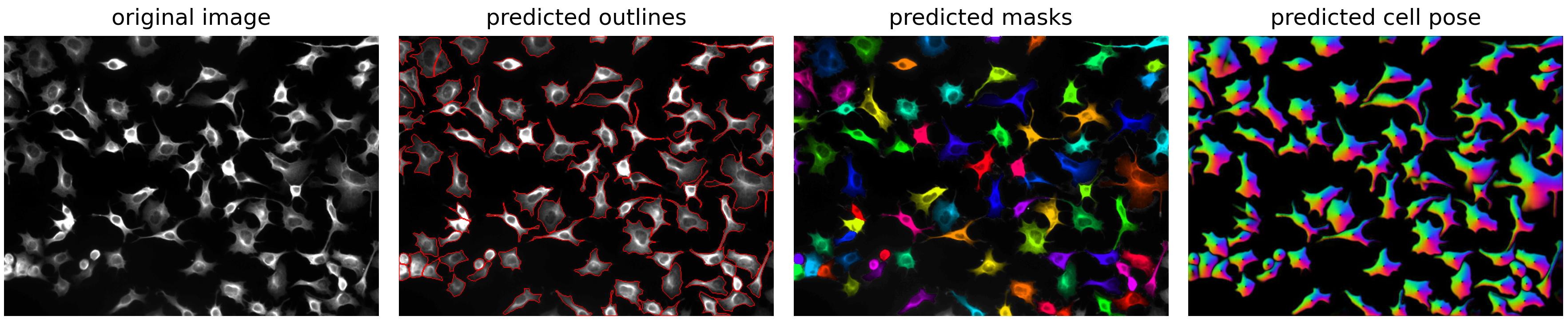
Display the Results#
fig = plt.figure(figsize=(12, 5))
plot.show_segmentation(fig, image[channel], masks, flows[0])
plt.tight_layout()
# Optional if you want to also save the figure
# plt.savefig(f"path/to/output/{Path(image_path).stem}_cp_output.png")
plt.show()
Run Cellpose on a Folder of Images#
Now that we’ve seen how to run Cellpose on a single image, let’s scale up and apply it to a folder of images. This is useful when you have an entire experiment or dataset that you want to segment automatically.
Cellpose provides a convenient built-in function for this: model.eval() can be used with a folder path, and it will process all compatible image files in that folder.
We’ll walk through how to:
Point Cellpose to your image directory
Choose the segmentation type (e.g., “nuclei” or “cyto”)
Set output options like saving masks and outlines
Visualize a few results to make sure everything worked
💡 Tip: Make sure your images are in
.tif,.png, or.jpgformat.
Let’s get started with folder-based segmentation!
folder_path = Path("data/05_segmentation_cellpose")

# Read file names
images = []
for f in folder_path.glob("*.tif"):
    images.append(f)
# same as running: files = [f for f in folder_path.glob("*.tif")]

# Cellpose parameters
flow_threshold = 0.4
cellprob_threshold = 0.0
tile_norm_blocksize = 0

# Run Cellpose on all images
for image_path in tqdm(images):
    image = tifffile.imread(image_path)
    masks, flows, styles = model.eval(
        image,
        batch_size=32,
        flow_threshold=flow_threshold,
        cellprob_threshold=cellprob_threshold,
        normalize={"tile_norm_blocksize": tile_norm_blocksize},
    )

    # Optional: display each image with its segmentation
    # fig = plt.figure(figsize=(12, 5))
    # plot.show_segmentation(fig, image, masks, flows[0])
    # plt.tight_layout()
    # plt.show()

    # Save the segmentation results
    output_path = folder_path / f"{image_path.stem}_labeled_mask.tif"
    tifffile.imwrite(output_path, masks.astype("uint16"))