Python for bioimage analysis

Download this Notebook Open in Colab

# /// script
# requires-python = ">=3.12"
# dependencies = [
#     "bioio",
#     "bioio-nd2",
#     "imageio",
#     "matplotlib",
#     "ndv[jupyter,vispy]",
#     "numpy",
#     "rich",
#     "tifffile",
# ]
# ///

Description

This notebook focuses on numpy arrays - the most common representation of images in python.

Numpy stands for Numerical Python. It lets us perform mathematical operations on numpy arrays.
A numpy array holds numeric data—such as images!
In short, numpy lets us compute on and manipulate images quickly.

Objectives

We learn how to read in images, manipulate them and visualize them as numpy arrays, and about common pitfalls.

Table of Contents

1. Importing libraries

2. Reading images using tifffile

3. View images using ndv

4. numpy: indexing

5. numpy: multiple channels and z-stacks

6. numpy: generating numpy arrays

7. Visualize images using matplotlib (functions)

8. Reading images using bioio

---

1. Import all necessary libraries

import matplotlib.pyplot as plt
import ndv
import numpy as np
import tifffile
from bioio import BioImage
from rich import print

2. Read an image using tifffile

stack_path = "../../_static/images/python4bia/confocal-series.tif"  # Specify the path to the image
stack = tifffile.imread(stack_path)  # read stack_path and store it in stack

print(type(stack))
print(stack.dtype)
print(stack.shape)

<class 'numpy.ndarray'>

uint8

(25, 2, 400, 400)

3. View images using ndv

ndv documentation: https://pyapp-kit.github.io/ndv/latest/
Reminder: we import ndv using

import ndv

ndv.imshow(stack)

snapshot

---

4. numpy arrays - intro, indexing and slicing

4.1 Load an image

We load the image cateye_nonsquare_ds.tif using tifffile.

cat_img_path = "../../_static/images/python4bia/cateye_nonsquare_ds.tif"
cat = tifffile.imread(cat_img_path)

4.2 Inspecting numpy arrays

Inspecting raw intensity values

Remember, the image is now a numpy array.

type(cat)

numpy.ndarray

The simplest way of viewing its intensity values is by running the following cell:

cat

array([[217, 176, 226, 253, 150, 226, 228, 220, 210, 218, 224],
       [215, 181, 236, 219, 225, 220, 215, 210, 141, 173, 105],
       [199, 140, 231, 222, 228, 238, 218, 194, 195, 197,  34],
       [206, 202, 236, 240, 213, 218, 192, 249, 244, 240,  52],
       [226, 220, 235, 202, 188,  50, 226, 242, 233, 224,  49],
       [238, 247, 208, 179, 234,  91, 181, 227, 237, 140,  45],
       [230, 164, 234, 176, 182, 233, 237, 209, 176,  51, 192],
       [246,  86, 204, 218, 199, 202, 230, 208,  51,  61, 222],
       [251,  34, 150, 201, 198, 223, 157,  57,  56, 239, 101],
       [249, 131, 111,  62,  48,  53,  67, 110, 223, 129, 140],
       [253, 148, 169, 184, 150, 182, 197, 236, 206, 142, 197],
       [253, 175, 202, 222, 253, 251, 234, 185, 165, 144, 164]],
      dtype=uint8)

Reminder: we use an alternative print function to print rich text.
We import it using:

from rich import print

print(cat)

[[217 176 226 253 150 226 228 220 210 218 224]
 [215 181 236 219 225 220 215 210 141 173 105]
 [199 140 231 222 228 238 218 194 195 197  34]
 [206 202 236 240 213 218 192 249 244 240  52]
 [226 220 235 202 188  50 226 242 233 224  49]
 [238 247 208 179 234  91 181 227 237 140  45]
 [230 164 234 176 182 233 237 209 176  51 192]
 [246  86 204 218 199 202 230 208  51  61 222]
 [251  34 150 201 198 223 157  57  56 239 101]
 [249 131 111  62  48  53  67 110 223 129 140]
 [253 148 169 184 150 182 197 236 206 142 197]
 [253 175 202 222 253 251 234 185 165 144 164]]

4.3 Inspecting properties of the image

Let’s print a few properties of cat

print(f"Type of the image: {type(cat)}")
print(f"Datatype of the image: {cat.dtype}")
print(f"Shape of the image: {cat.shape}")  # Dimensions of the image
print(f"Minimum pixel value: {cat.min()}")  # Min pixel value
print(f"Maximum pixel value: {cat.max()}")  # Max pixel value
print(f"Mean pixel value: {cat.mean():.2f}")  # Average pixel value

Type of the image: <class 'numpy.ndarray'>

Datatype of the image: uint8

Shape of the image: (12, 11)

Minimum pixel value: 34

Maximum pixel value: 253

Mean pixel value: 184.17

4.4 Generate a simple plot of the image

Reminder: we import plt using

import matplotlib.pyplot as plt

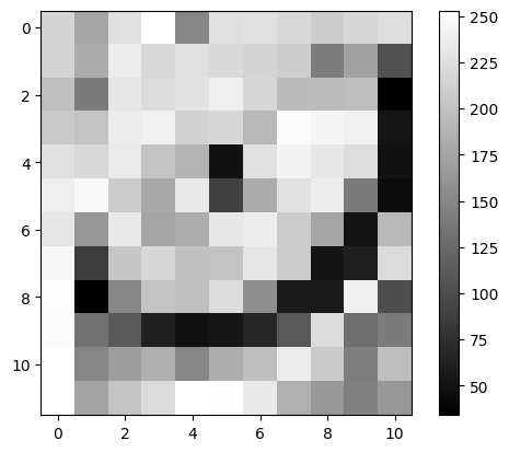
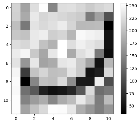
Plot using plt.imshow()

✍️ Exercise: Code along

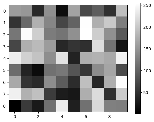
plt.imshow(cat, cmap="gray")
plt.colorbar()
plt.show()

✍️ Exercise: Write a plotting function

Write the previous plotting code as a function

def simpleplot(image: np.ndarray) -> None:
    """
    Plot `image` in grayscale with an accompanying colorbar.

    Parameters
    ----------
    image : A 2D np.ndarray
    """
    plt.imshow(image, cmap="gray")
    plt.colorbar()
    plt.show()

simpleplot(cat)

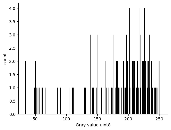
4.5 Plot a simple histogram

Show code cell content

Hide code cell content

def valueplot(image: np.ndarray, indices: str = "empty", fontsize: int = 10) -> None:
    """
    Show a 2-D array as a grayscale heat-map, print each pixel's value on top,
    and optionally outline pixels or regions.

    Parameters
    ----------
    image : np.ndarray
        Array of shape (rows, cols).
    indices : str, optional
        String with numpy indexing notation using either brackets [] or parentheses ().

        Examples:
        - "(5, 3)" or "[5, 3]" - single pixel
        - "[0:5, 3:7]" or "(0:5, 3:7)" - region from rows 0-4, columns 3-6
        - "(:, 0)" or "[:, 0]" - entire column 0
        - "(2, :)" or "[2, :]" - entire row 2
        - "[:,:]" - entire image
        - "[::2, 1::3]" - every 2nd row, every 3rd column starting from column 1
    """

    if indices == "empty":
        indices = "[0:0, 0:0]"

    def parse_index_string(index_str: str) -> tuple:
        """Parse numpy-style indexing string into tuple of slices/ints."""
        # Remove brackets and parentheses
        index_str = index_str.strip()
        if index_str.startswith("[") and index_str.endswith("]"):
            index_str = index_str[1:-1]
        elif index_str.startswith("(") and index_str.endswith(")"):
            index_str = index_str[1:-1]

        # Split by comma
        parts = [part.strip() for part in index_str.split(",")]

        if len(parts) != 2:
            raise ValueError(
                "Index string must have exactly 2 parts separated by comma"
            )

        result = []
        for part in parts:
            if part == ":" or part == "":
                # Full slice
                result.append(slice(None))
            elif ":" in part:
                # Parse slice notation
                slice_parts = part.split(":")
                start = None if slice_parts[0] == "" else int(slice_parts[0])
                stop = (
                    None
                    if len(slice_parts) < 2 or slice_parts[1] == ""
                    else int(slice_parts[1])
                )
                step = (
                    None
                    if len(slice_parts) < 3 or slice_parts[2] == ""
                    else int(slice_parts[2])
                )
                result.append(slice(start, stop, step))
            else:
                # Single integer
                result.append(int(part))

        return tuple(result)

    if indices is None:
        indices = [None, None]
    else:
        # Parse string notation
        indices = parse_index_string(indices)

    plt.imshow(image, cmap="gray", vmin=np.min(image), vmax=np.max(image))

    # Annotate each pixel with its value
    for i in range(image.shape[0]):  # row
        for j in range(image.shape[1]):  # column
            plt.text(
                j,
                i,
                str(image[i, j]),
                ha="center",
                va="center",
                color="magenta",
                fontsize=fontsize,
            )

    plt.ylabel("row; y; axis = 0", fontsize=fontsize)
    plt.xlabel("column; x; axis = 1", fontsize=fontsize)

    # Handle different types of indices
    if indices is not None and len(indices) == 2:
        row_idx, col_idx = indices

        # Convert indices to ranges for highlighting
        if isinstance(row_idx, slice):
            # Handle slice objects
            start_row = row_idx.start if row_idx.start is not None else 0
            stop_row = row_idx.stop if row_idx.stop is not None else image.shape[0]
            step_row = row_idx.step if row_idx.step is not None else 1

            if start_row < 0:
                start_row = image.shape[0] + start_row
            if stop_row < 0:
                stop_row = image.shape[0] + stop_row
            row_range = list(range(start_row, min(stop_row, image.shape[0]), step_row))
        elif isinstance(row_idx, int):
            # Single row
            if row_idx < 0:
                row_idx = image.shape[0] + row_idx
            row_range = [row_idx] if 0 <= row_idx < image.shape[0] else []
        else:
            row_range = list(range(image.shape[0]))  # All rows if None or invalid

        if isinstance(col_idx, slice):
            # Handle slice objects
            start_col = col_idx.start if col_idx.start is not None else 0
            stop_col = col_idx.stop if col_idx.stop is not None else image.shape[1]
            step_col = col_idx.step if col_idx.step is not None else 1

            if start_col < 0:
                start_col = image.shape[1] + start_col
            if stop_col < 0:
                stop_col = image.shape[1] + stop_col
            col_range = list(range(start_col, min(stop_col, image.shape[1]), step_col))
        elif isinstance(col_idx, int):
            # Single column
            if col_idx < 0:
                col_idx = image.shape[1] + col_idx
            col_range = [col_idx] if 0 <= col_idx < image.shape[1] else []
        else:
            col_range = list(range(image.shape[1]))  # All columns if None or invalid

        # Highlight the region
        for row in row_range:
            for col in col_range:
                rect = plt.Rectangle(
                    (col - 0.5, row - 0.5),
                    1,
                    1,
                    linewidth=2,
                    edgecolor="yellow",
                    facecolor="none",
                )
                plt.gca().add_patch(rect)

    plt.yticks(list(range(image.shape[0])))
    plt.xticks(list(range(image.shape[1])))
    plt.tight_layout()
    plt.show()

✍️ Exercise: Code along

plt.hist(cat.ravel(), bins=256, color="k")
plt.xlabel(f"Gray value {cat.dtype}")  # format string
plt.ylabel("count")

Text(0, 0.5, 'count')

---

4.6 Indexing: individual entries

In this 2D array, the first number indexes axis 0. The second number indexes axis 1.

first entry	second entry
axis 0	axis 1
row	column

# Pass numbers directly
print(cat[0, 10])

224

Tip: We can pass variables instead of numbers if the same indices are to be reused:

# Define variables
row, col = 0, 10
print(cat[row, col])

224

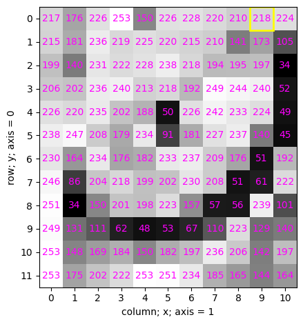
✍️ Exercise: Enter different values for row and col:

valueplot is a costumn function that visualizes indices provided as strings

row, col = 0, -2
valueplot(cat, indices=str([row, col]))

4.7 Indexing: Rows and columns

Rows

row = 1
print(cat[row, :])  #
print(cat[row,])  # This is equivalent to the above
print(cat[row])  # If only one number is supplied, it applies to axis 0

[215 181 236 219 225 220 215 210 141 173 105]

[215 181 236 219 225 220 215 210 141 173 105]

[215 181 236 219 225 220 215 210 141 173 105]

Columns

✍️ Exercise: Uncomment the cell below and run it.

If there’s an error, can we fix it by adding one symbol only?

# print(cat[1, ]) # Tries to print the first row
# print(cat[, 1]) # Tries to print the first column

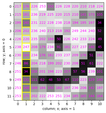
✍️ Exercise: Highlight either a full row or a full column

Experiment with different entries.

valueplot(cat, indices="[:, 1]")

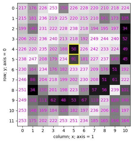
✍️ Exercise:

Highlight these values using function valueplot()

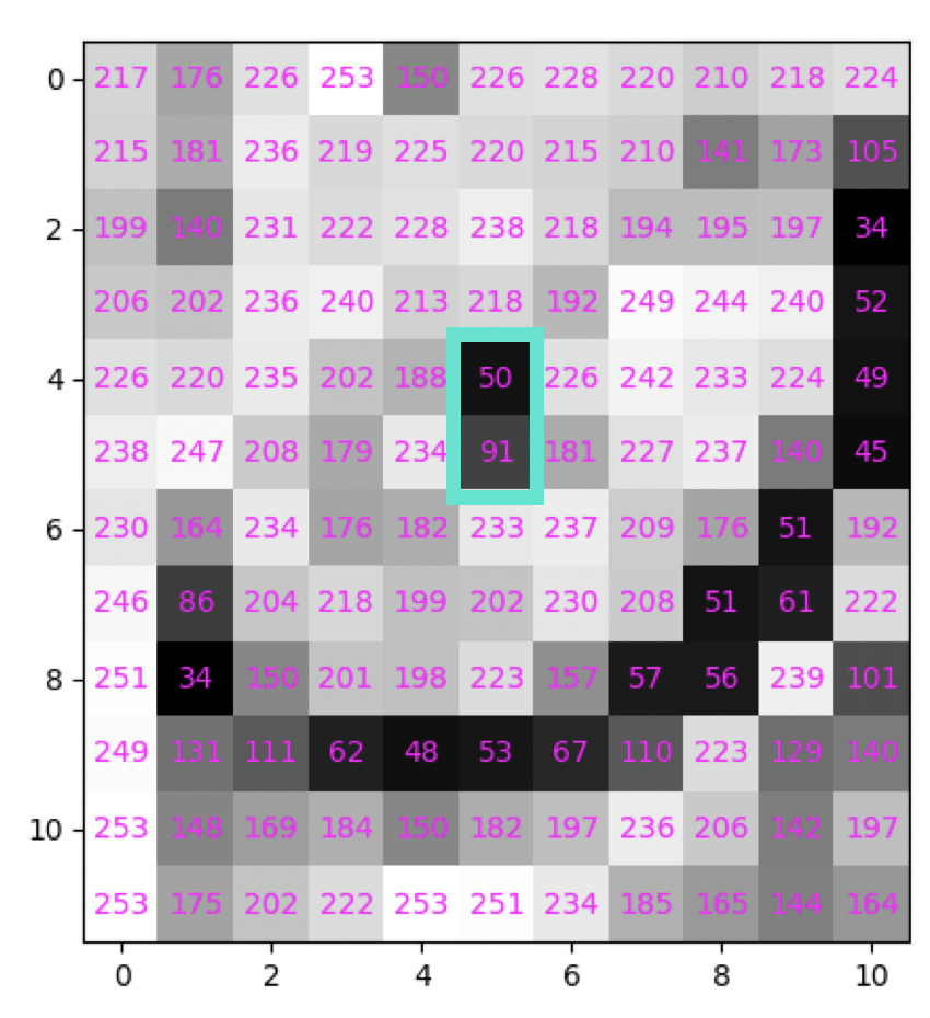
valueplot(cat, "[4:6, 5]")

4.8 Modifying intensity values using indexing

✍️ Exercise: Make a copy of cat, and name it lazercat (new variable). Assign a value of 255 to the indicated pixels

### Pitfall
lazercat = cat
lazercat[4:6, 5] = 255
simpleplot(cat)

✍️ Exercise: Inspect the pixelvalues of cat and lazercat using simpleplot()

simpleplot(cat)
simpleplot(lazercat)

# reload cat in case it was overwritten
def load_cat(cat_img_path) -> np.ndarray:
    cat = tifffile.imread(cat_img_path)
    return cat


cat = load_cat(cat_img_path)

lazercat = cat.copy()
lazercat[4:6, 5] = 255

simpleplot(cat)
simpleplot(lazercat)

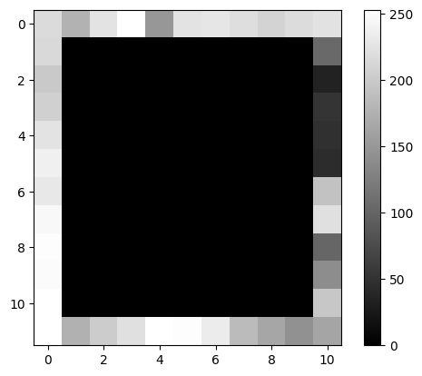
✍️ Exercise: Make a copy of cat and name it pirate. Assign to all pixels but the rim-pixels a value of 0. Plot to verify!

# cat = load_cat(cat_img_path) # Run if you accidentally overwrote ```cat```

pirate = cat.copy()
pirate[1:-1, 1:-1] = 0
simpleplot(pirate)

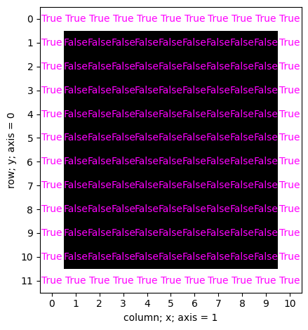
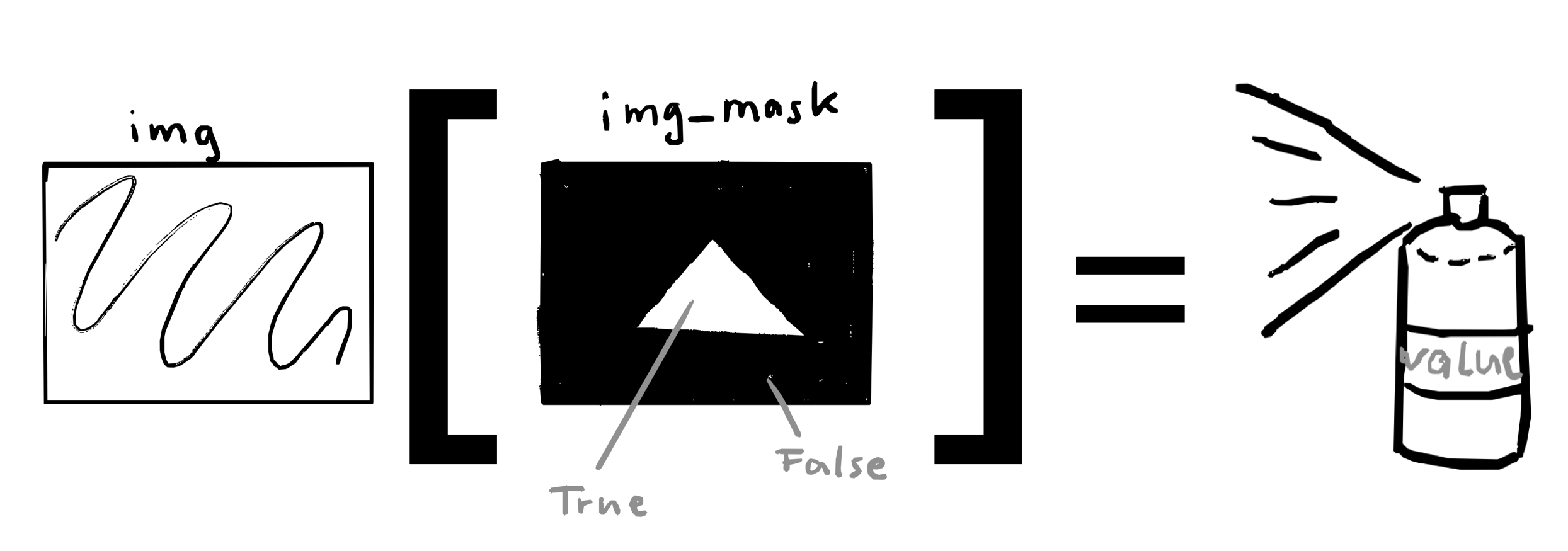
4.9 Boolean indexing

Show code cell content

Hide code cell content

monocle_bool = np.array(cat, dtype=bool)
monocle_bool[0, :] = False
monocle_bool[-1, :] = False
monocle_bool[:, 0] = False
monocle_bool[:, -1] = False
monocle_bool = ~monocle_bool

monocle_bool is a 2D numpy array of the same dimensions as cat.
Instead of integer intensity values, its pixel-values are either True or False.
Let’s inspect monocle_bool

print(monocle_bool.dtype)
print(monocle_bool.shape)
valueplot(monocle_bool)

bool

(12, 11)

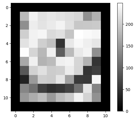
✍️ Exercise: monocle is a copy of cat. Use monocle_bool to assign a value of 0 to the rim pixels of monocle. Plot to verify

# cat = load_cat(cat_img_path) # Run if you accidentally overwrote ```cat```

monocle = cat.copy()

Tip:

monocle[monocle_bool] = 0  # Set rim pixels to 0
simpleplot(monocle)

---

5. numpy and multichannel/z-stacks

Reminder: Previously, we loaded a 2-channel z-stack and named it stack

stack = tifffile.imread(stack_path)

# Here, we define a function to read the stack from a specified path
def read_stack(
    path: str = stack_path,
) -> np.ndarray:
    stack = tifffile.imread(path)
    return stack

stack = read_stack(
    stack_path
)  # reloads image "stack". Run this if you accidentally overwrote `stack`

print(stack.dtype)
print(stack.shape)

uint8

(25, 2, 400, 400)

Reminder: We can use ndv to inspect an image

ndv.imshow(stack)

snapshot

✍️ Exercise: Create a numpy array ch0 that contains the first channel of stack

Bonus: Create a numpy array ch1 that contains the second channel of stack.
Note: This is 0-indexed!

# Reminder
stack.shape

(25, 2, 400, 400)

ch0 = stack[:, 0].copy()
ch1 = stack[:, 1].copy()

print(ch0.shape)

(25, 400, 400)

✍️ Exercise: plot ch0 using function simpleplot()

## Pitfall:
# simpleplot(ch0)

# simpleplot can only plot a 2D array.
# You must index ch0 such that it returns a 2D array. Examples:
z = 17

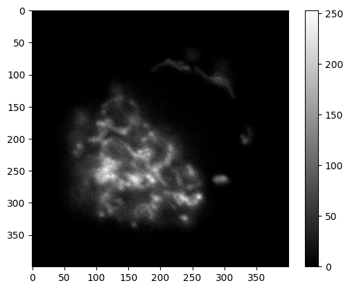
simpleplot(ch0[z])  # show only one z-plane

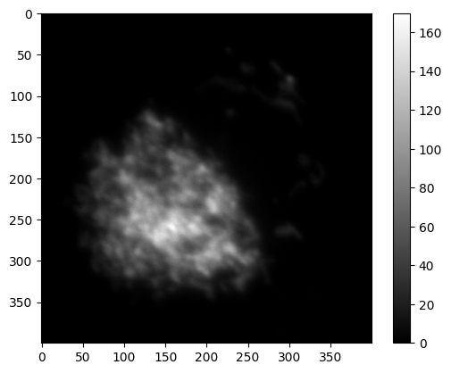
✍️ Exercise: Create a mean-projection of channel ch0

Objective
Convert the 3-D stack ch0 (shape (Z, 400, 400)) into a 2-D image by averaging over its z-planes.

Quick reference numpy.mean:

numpy.mean(a, axis=None, dtype=None, out=None, keepdims=<no value>, *, where=<no value>)

a (array_like) – Array containing numbers whose mean is desired. If a is not an array, a conversion is attempted.
axis (int, tuple[int], or None) – Axis or axes along which the means are computed. The default is to compute the mean of the flattened array.

# mean_project_ch0 = ...  # fill in the gaps
# print(mean_project_ch0.shape)
# simpleplot(mean_project_ch0)

mean_project_ch0 = np.mean(ch0, axis=0)
print(mean_project_ch0.shape)
simpleplot(mean_project_ch0)

(400, 400)

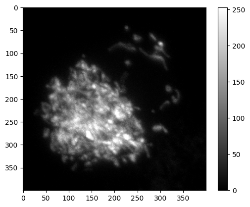
✍️ Exercise: compute the max projection of ch0

Collapse ch0 into a 2D image by only displaying the maximum value along z. The result should be a (400, 400) array where each value represents the maximum of the all z intensity values at that position.
This is called max projection.

https://numpy.org/doc/2.2/reference/generated/numpy.max.html#numpy-max

max_project_ch0 = np.max(ch0, axis=0)
print(max_project_ch0.shape)
simpleplot(max_project_ch0)

(400, 400)

✍️ Exercise (bonus): Try other numpy projections

Below are a few operations taken from https://numpy.org/doc/2.2/reference/routines.statistics.html

Category	Function	What it does along an axis	Example projection (axis=0)
Order statistics	np.percentile	q-th percentile	p50 = np.percentile(stack, 50, axis=0) (numpy.org)
	np.quantile	q-th quantile (fraction 0-1)	q25 = np.quantile(stack, 0.25, axis=0) (numpy.org)
Averages & variances	np.median	Median	med = np.median(stack, axis=0) (numpy.org)
	np.average	Weighted average (pass weights=)	w_avg = np.average(stack, axis=0, weights=w) (numpy.org)
	np.mean	Arithmetic mean	mean = np.mean(stack, axis=0) (numpy.org)
	np.std	Standard deviation	sigma = np.std(stack, axis=0) (numpy.org)
	np.var	Variance	var_map = np.var(stack, axis=0) (numpy.org)

# Write your code here

---

6. Generating numpy arrays

There are many reasons to generate numpy arrays

• We may need it as a basis for further computations

• We want to generate dummy data to test functions, etc

Create an array of filled with 0s with shape [5, 5]

zero_array = np.zeros([5, 5])
print(zero_array)
zero_array.dtype

[[0. 0. 0. 0. 0.]
 [0. 0. 0. 0. 0.]
 [0. 0. 0. 0. 0.]
 [0. 0. 0. 0. 0.]
 [0. 0. 0. 0. 0.]]

dtype('float64')

Generate an array of zeroes that has the same properties as cat

zeroes_cat = np.zeros_like(cat)

print(zeroes_cat)
print(zeroes_cat.shape)
print(zeroes_cat.dtype)

[[0 0 0 0 0 0 0 0 0 0 0]
 [0 0 0 0 0 0 0 0 0 0 0]
 [0 0 0 0 0 0 0 0 0 0 0]
 [0 0 0 0 0 0 0 0 0 0 0]
 [0 0 0 0 0 0 0 0 0 0 0]
 [0 0 0 0 0 0 0 0 0 0 0]
 [0 0 0 0 0 0 0 0 0 0 0]
 [0 0 0 0 0 0 0 0 0 0 0]
 [0 0 0 0 0 0 0 0 0 0 0]
 [0 0 0 0 0 0 0 0 0 0 0]
 [0 0 0 0 0 0 0 0 0 0 0]
 [0 0 0 0 0 0 0 0 0 0 0]]

(12, 11)

uint8

✍️ Exercise: Code along: simulate a multichannel image

• Call it dual_ch_fake

• Of shape [2,9,10]

• dtype is np.uint8

• Each pixel has a random value between 0 (inclusive) and 256 (exclusive)

?np.random.randint
# dual_ch_fake = np.random.randint(..., dtype=np.uint8))

dual_ch_fake = np.random.randint(0, 256, size=(2, 9, 10), dtype=np.uint8)

Let’s plot the two channels:

simpleplot(dual_ch_fake[0, :, :])

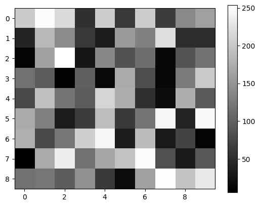
simpleplot(dual_ch_fake[1, :, :])

✍️ Exercise (Bonus): Check whether np.mean does what you expect it to do without using numpy operations

Reminder: We can calculate a mean image of the two channels like this:

mean_of_channels = np.mean(dual_ch_fake, axis=0)

And generate an array of each channel like this:

ch_0 = dual_ch_fake[0, :, :].copy()
ch_1 = dual_ch_fake[1, :, :].copy()

And compare two elements like this:

a = 5
b = 5
a == b

True

### Pitfall
mean_of_channels == (ch_0 + ch_1) / 2  # integer overflow

array([[False,  True,  True, False, False,  True,  True,  True,  True,
         True],
       [False, False,  True,  True, False,  True,  True, False, False,
        False],
       [ True, False,  True, False,  True,  True,  True, False,  True,
        False],
       [ True,  True,  True,  True, False, False, False, False, False,
         True],
       [ True,  True, False, False, False,  True, False, False, False,
         True],
       [ True, False,  True, False, False,  True, False, False,  True,
         True],
       [False, False,  True,  True, False,  True, False, False,  True,
        False],
       [False,  True, False,  True,  True,  True, False,  True,  True,
         True],
       [False,  True,  True,  True, False, False, False,  True, False,
         True]])

### Possible solution:
mean_manual = dual_ch_fake[0, :, :] / 2 + dual_ch_fake[1, :, :] / 2
print(mean_of_channels == mean_manual)
print(np.unique(mean_of_channels == mean_manual))

[[ True  True  True  True  True  True  True  True  True  True]
 [ True  True  True  True  True  True  True  True  True  True]
 [ True  True  True  True  True  True  True  True  True  True]
 [ True  True  True  True  True  True  True  True  True  True]
 [ True  True  True  True  True  True  True  True  True  True]
 [ True  True  True  True  True  True  True  True  True  True]
 [ True  True  True  True  True  True  True  True  True  True]
 [ True  True  True  True  True  True  True  True  True  True]
 [ True  True  True  True  True  True  True  True  True  True]]

[ True]

Conclusion: Where possible, use numpy operations instead of writing your own operations!

---

7. Visualization using matplotlib

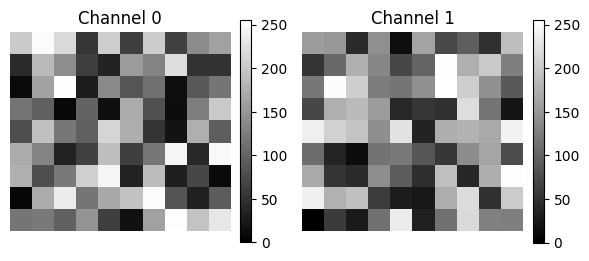
def show_2_channels(image: np.ndarray, figsize: tuple = (6, 3)) -> None:
    """
    Show a 2-channel image with each channel in a separate subplot.
    Parameters
    ----------
    image : np.ndarray
        A 3D array of shape (2, height, width) representing a 2-channel image.
    Each channel is expected to be a 2D array of pixel values.
    """
    fig, axes = plt.subplots(1, 2, figsize=figsize)

    for i in range(2):
        im = axes[i].imshow(image[i, :, :], cmap="gray", vmin=0, vmax=255)
        axes[i].imshow(image[i, :, :], cmap="gray", vmin=0, vmax=255)
        axes[i].set_title(f"Channel {i}")
        axes[i].axis("off")
        # Add colorbar for this subplot
        fig.colorbar(im, ax=axes[i], fraction=0.046, pad=0.04)

    plt.tight_layout()
    plt.show()

Let’s test the function using dual_ch_fake that we previously generated

show_2_channels(dual_ch_fake)

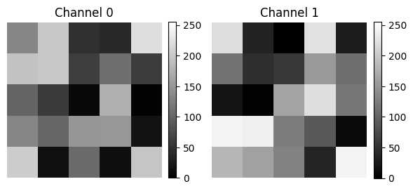
✍️ Exercise: plot all channels of the following image. Write a function show_all_channels().

threechannel = np.random.randint(0, 256, size=(3, 5, 5), dtype=np.uint8)

threechannel.shape

(3, 5, 5)

# This works, but it will only show the first two channels.
show_2_channels(threechannel)

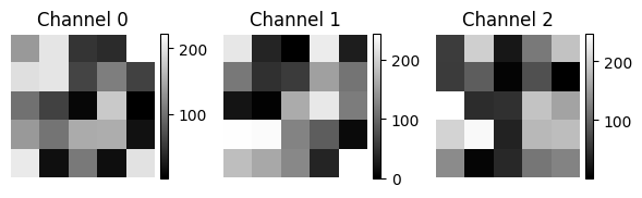
def show_all_channels(
    image: np.ndarray, nchannels: int | None = None, figsize: tuple = (6, 3)
) -> None:
    """
    Show all channels of a multi-channel image.
    Parameters
    ----------
    image : np.ndarray
        A 3D array of shape (nchannels, height, width) representing a multi-channel image.
    Each channel is expected to be a 2D array of pixel values.
    nchannels : int, optional
        The number of channels in the image. If None, it will be inferred from the shape
        of the image.
    figsize : tuple, optional
        The size of the figure to display the channels. Default is (6, 3).
    """
    if not nchannels:
        nchannels = image.shape[0]

    fig, axes = plt.subplots(1, nchannels, figsize=figsize)
    for i in range(nchannels):
        vmax = np.max(image[i, :, :])
        vmin = np.min(image[i, :, :])
        im = axes[i].imshow(
            image[i, :, :],
            cmap="gray",
            vmin=vmin,
            vmax=vmax,
        )
        axes[i].imshow(image[i, :, :], cmap="gray", vmin=vmin, vmax=vmax)
        axes[i].set_title(f"Channel {i}")
        axes[i].axis("off")

        # Add colorbar for this subplot
        fig.colorbar(im, ax=axes[i], fraction=0.046, pad=0.04)

    plt.tight_layout()
    plt.show()

show_all_channels(threechannel)

---

8. Bonus: read images using bioio

bioio can read various image file formats

There are many ways of reading image files. bioio can read images of different file-formats.
Different fileformats require different plugins

Plug-in	Extension	Repository
arraylike	ArrayLike	Built-In
bioio-czi	.czi	Repo
bioio-dv	.dv, .r3d	Repo
bioio-imageio	.jpg, .png, Full List	Repo
bioio-lif	.lif	Repo
bioio-nd2	.nd2	Repo
bioio-ome-tiff	.ome.tiff, .tiff	Repo
bioio-ome-tiled-tiff	.tiles.ome.tif	Repo
bioio-ome-zarr	.zarr	Repo
bioio-sldy	.sldy, .dir	Repo
bioio-tifffile	.tif , .tiff	Repo
bioio-tiff-glob	.tiff (glob)	Repo
bioio-bioformats	Full List	Repo

We use bioio-nd2 to read an nd2 file.

Example: Read an nd2 file using bioio

bioio documentation: https://bioio-devs.github.io/bioio/OVERVIEW.html
Reminder: we import the relevant packages using

from bioio import BioImage
import bioio-nd2

bioio loads the image and metadata into a container. We name the container img

nd2_path = "../../_static/images/python4bia/single_pos_002.nd2"
img = BioImage(nd2_path)

type(img)

bioio.bio_image.BioImage

✍️ Exercise: Inspect properties of img

Below are a few examples of how to show properties of img taken from here.
Execute a few of them

# Get a BioImage object
img = BioImage("my_file.tiff")  # selects the first scene found
img.data  # returns 5D TCZYX ```numpy``` array
img.xarray_data  # returns 5D TCZYX xarray data array backed by numpy
img.dims  # returns a Dimensions object
img.dims.order  # returns string "TCZYX"
img.dims.X  # returns size of X dimension
img.shape  # returns tuple of dimension sizes in TCZYX order
img.get_image_data("CZYX", T=0)  # returns 4D CZYX numpy array

print(img.dims.order)
print(img.dims)
print(img.shape)

TCZYX

<Dimensions [T: 1, C: 3, Z: 1, Y: 2044, X: 2048]>

(1, 3, 1, 2044, 2048)

Extract a numpy array from the BioImage object

numpy documentation

Reminder: we import numpy as follows:

import numpy as np

# the image is contained in img.data
cells = img.data

type(cells)  # verify it's a numpy array

numpy.ndarray

cells.dtype  # check the datatype

dtype('uint16')

Inspect dimensions of stack

print(img.dims)  # Reminder:
print(cells.shape)  # only one time-point. This is like a movie with only one frame!

<Dimensions [T: 1, C: 3, Z: 1, Y: 2044, X: 2048]>

(1, 3, 1, 2044, 2048)

Use .squeeze() to remove axes of length one

To test these concepts, we first generate an array without an axis of size one:

simple_list = [1, 2, 3]
simple_array = np.array(simple_list)  # Turn the list into a numpy array

# print a few properties of simple_array
print(type(simple_array))
print(simple_array)
print(simple_array.shape)

<class 'numpy.ndarray'>

[1 2 3]

(3,)

Now, generate an array with an axis of length one:

nested_list = [[1, 2, 3]]  # There's extra brackets!
nested_array = np.array(nested_list)

# print a few properties of nested_array
print(type(simple_array))
print(nested_array)
print(nested_array.shape)

<class 'numpy.ndarray'>

[[1 2 3]]

(1, 3)

Next, .squeeze() removes axes of length one:

nested_array_squeezed = nested_array.squeeze()

# print a few properties of nested_array_squeezed
print(type(nested_array_squeezed))
print(nested_array_squeezed)
print(nested_array_squeezed.shape)

<class 'numpy.ndarray'>

[1 2 3]

(3,)

✍️ Exercise: apply this to image cells and print its shape

cells = cells.squeeze()
print(cells.shape)

(3, 2044, 2048)

Congratulations! cells is now in the correct format to be viewed and modified!

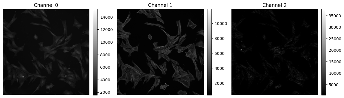
✍️ Exercise: Plot cells

# previously, we ran show_all_channels() on threechannel. Compare cells and threechannel:
print(cells.shape)
print(cells.dtype)
print(threechannel.shape)
print(threechannel.dtype)

(3, 2044, 2048)

uint16

(3, 5, 5)

uint8

show_all_channels(cells, figsize=(12, 6))