
Ilastik for Pixel Classification#
In this section, we will explore how to use Ilastik for semantic segmentation through pixel classification. This process involves training a machine learning model to classify pixels in an image based on user-defined labels.
In this exercise, we will use the pixel classification dataset of nuclei images, and the goal is to train a classifier to distinguish between nuclei and background.
What is Pixel Classification?#
Pixel classification is a fundamental image analysis technique that involves assigning a specific category or class to each pixel in an image based on its unique features, such as color, intensity, or texture. This approach is particularly valuable in tasks like semantic segmentation, where the objective is to divide an image into meaningful regions by categorizing pixels into predefined classes, such as background, foreground, or distinct objects.
Ilastik Pixel Classification Workflow#
For a detailed workflow instruction, you can refer to the Ilastik Pixel Classification Documentation.
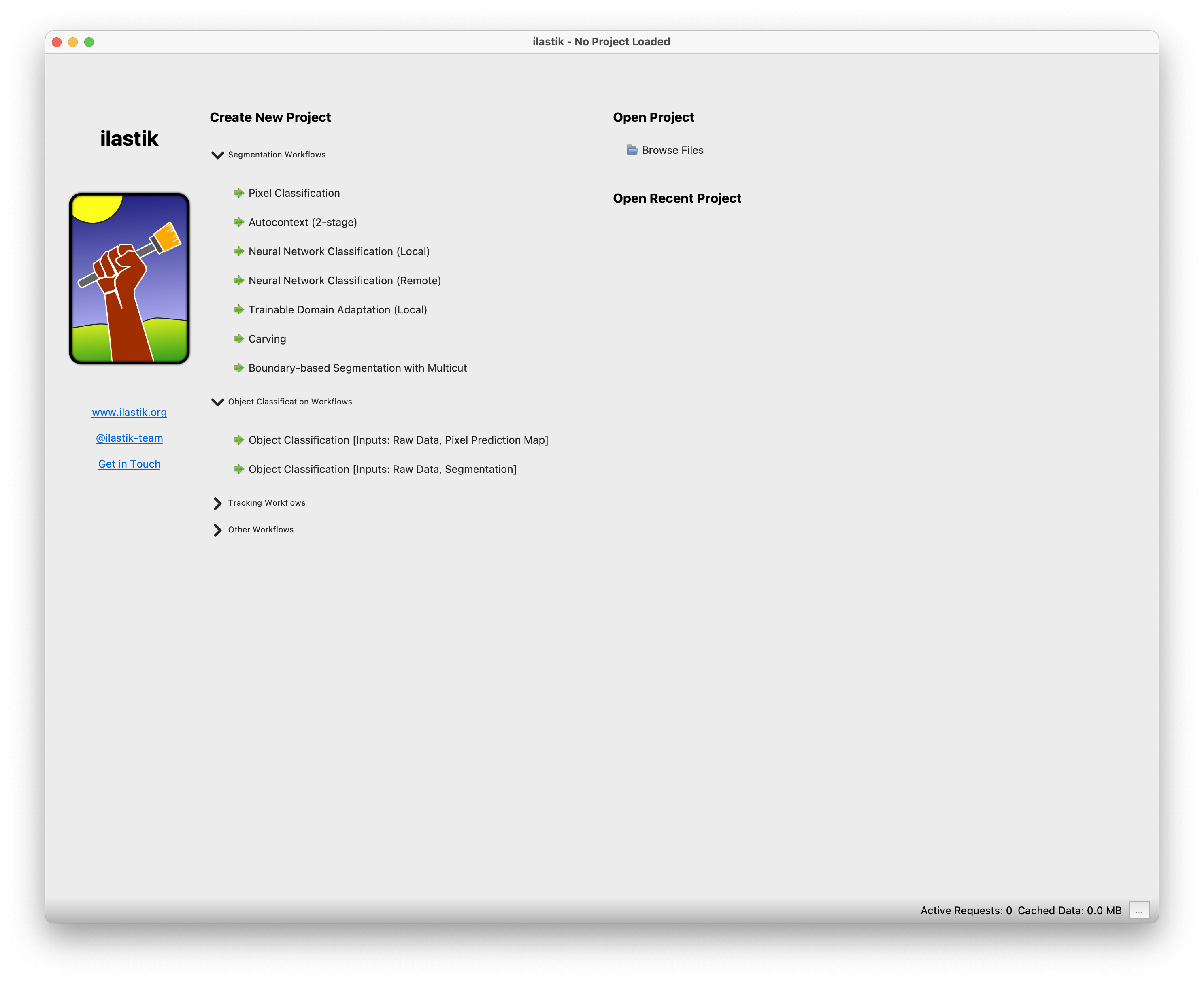
1. Select the Workflow#
When you open Ilastik, you will see the Startup Screen with various workflows. Select the Pixel Classification workflow by clicking on it. You will be automatically brought to the Input Data step.
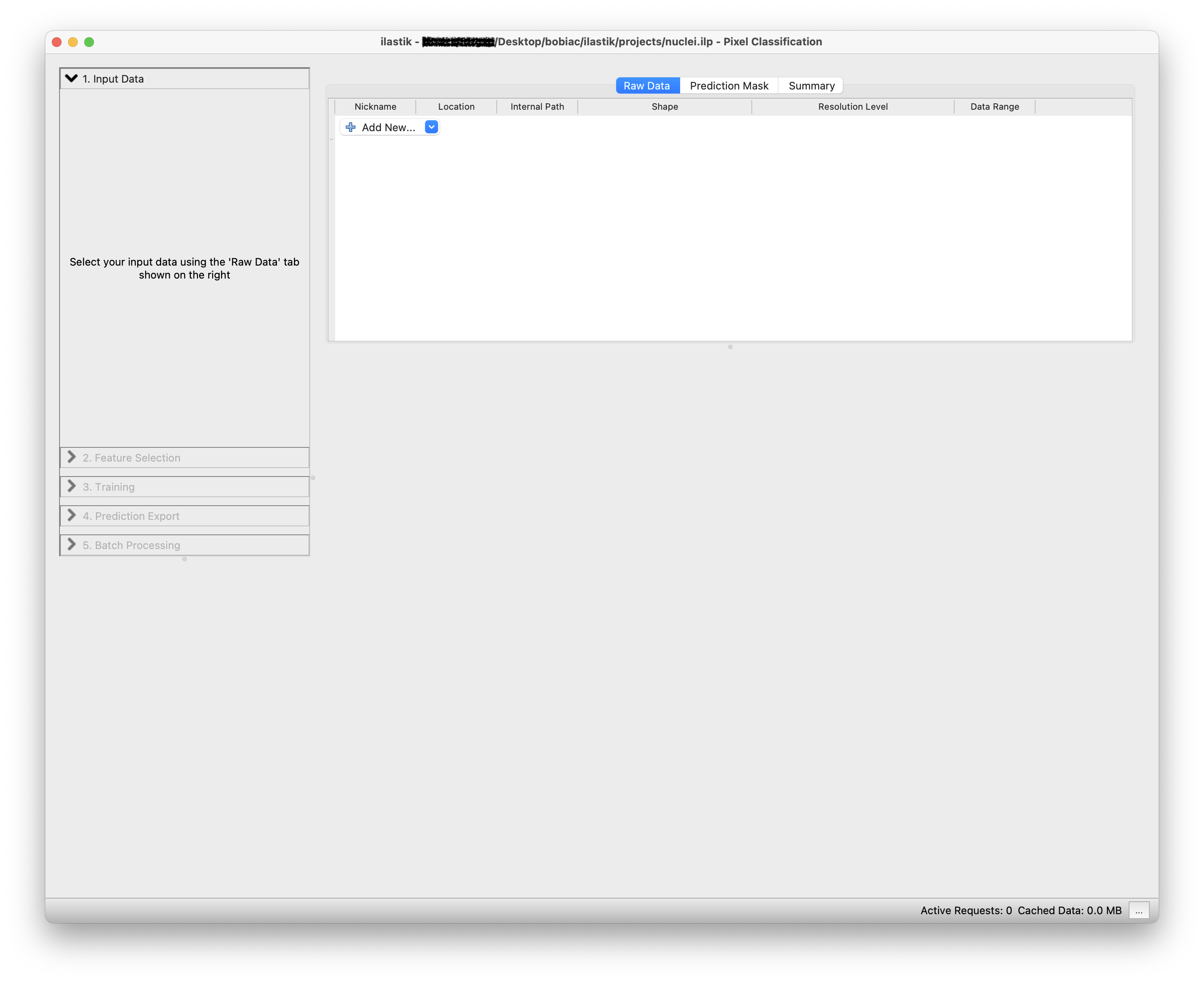
2. Load the Image Data#
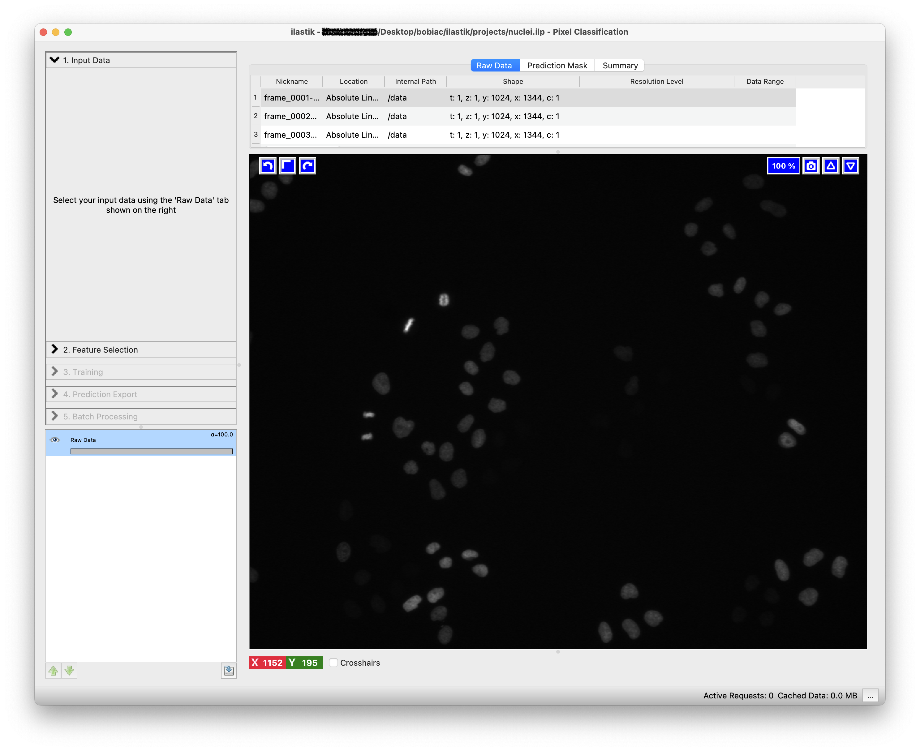
Next, you will need to load the image data you want to use to train the classifier. Select the Raw Data tab and either Drag and drop your image files into the Add New… field of the data table, or click on it to select your images. To create a robust classifier, you should load multiple images from the dataset. For this exercise, you can load 3 random images from the pixel classification dataset.
Once loaded, you can view the images by clicking on the image name in the data table. The corresponding image will be displayed in the window viewer.
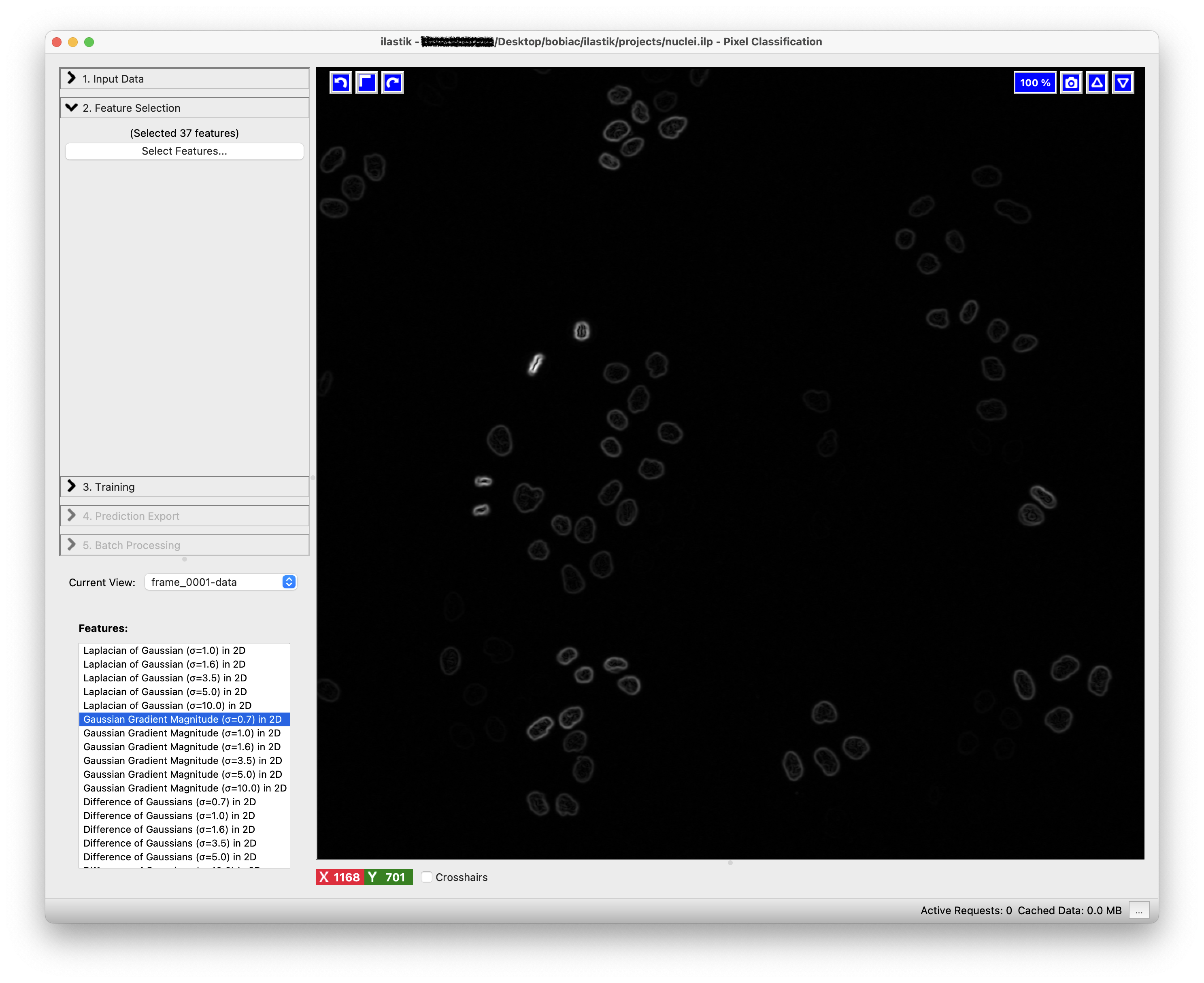
3. Select the Features#
To continue, click on the Feature Selection step (on the left side of the GUI) and then on the Select Features… button. Here, you can select the features and their scales (how much) that will be used to discriminate between the different classes of pixels.
For pixel classification, Ilastik provides a list of features types, divided by Color/Intensity, Edge, and Texture:
Color/Intensity: these features should be selected if the color or brightness can be used to discern objects
Edge: should be selected if brightness or color gradients can be used to discern objects.
Texture: this might be an important feature if the objects in the image have a special textural appearance.
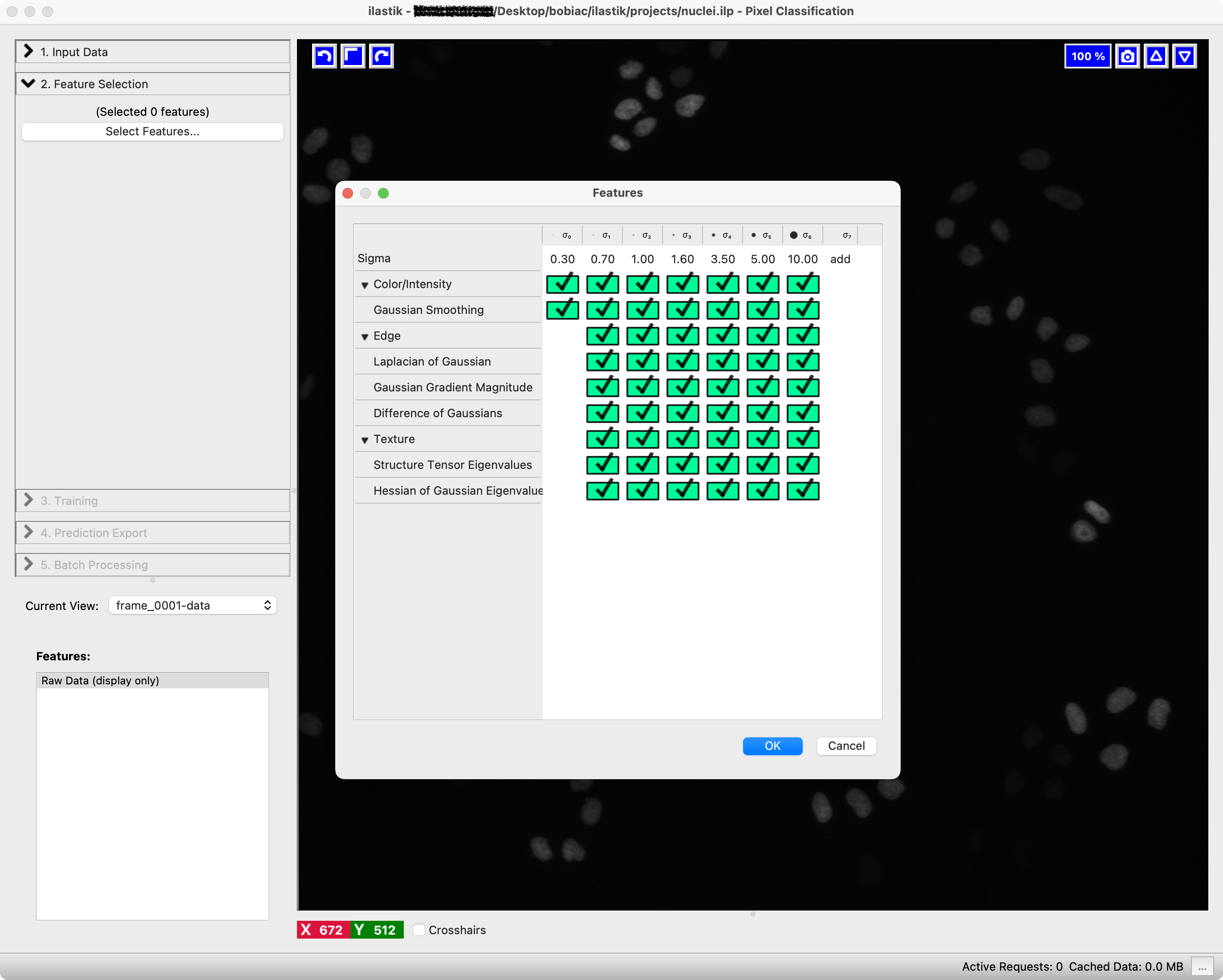
You can also choose the scale for each of these features. The scales correspond to the sigma of the Gaussian which is used to smooth the image before application of the filter. Filters with larger sigmas can thus pull in information from larger neighborhoods, but average out the fine details.
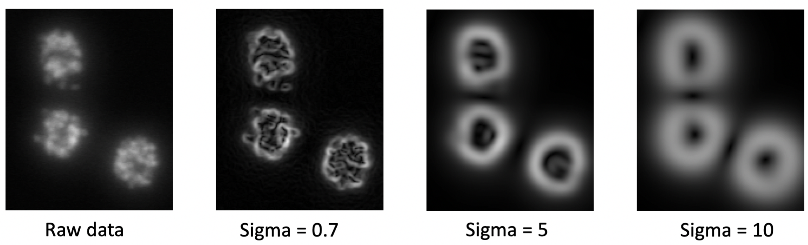
After clicking on Ok, you can visualize the effect of the selected features by clicking on one of the options in the Features list in the bottom left part of the GUI. This will help you understand if the selected features are suitable for your dataset. You can always go back to the Feature Selection step to change the features and their scales.
4. Train the Classifier#
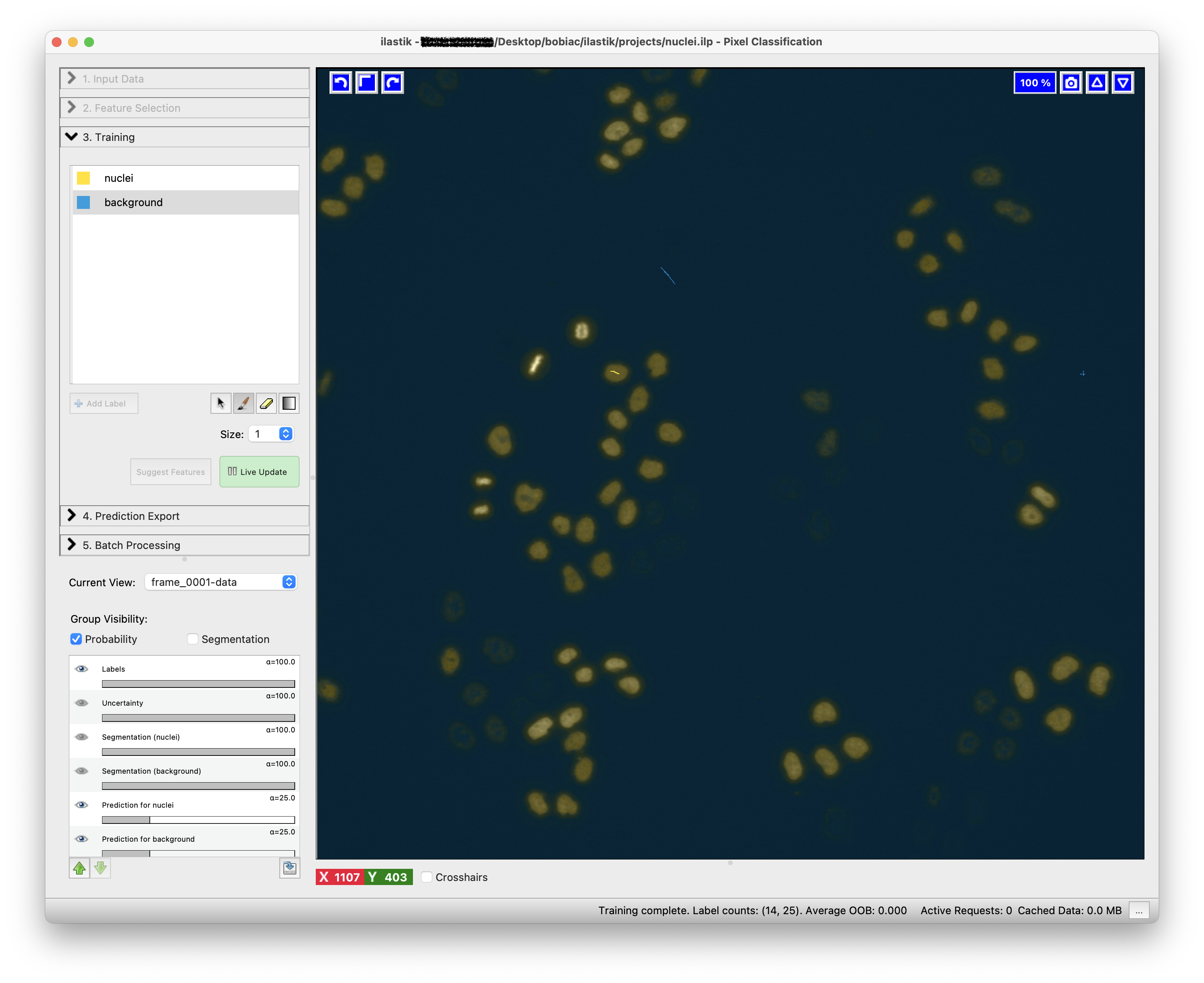
The next step is to train the classifier based on the features you selected. This is an interactive process where you will need to label a few pixels in the image with annotations to provide the classifier with examples of the different classes.
In the Training step (on the left side of the GUI) you can add, remove or edit the classes (labels) that you want to use for the classification. For this exercise, we will use two classes: nuclei and background. To rename the default classes, Label 1 and Label 2, double-click on each class and type the new name (You can also change the class color by double-clicking on the color box next to the class name).
Now you can start by choosing few pixels in the image that correspond to the nuclei class; select the nuclei class, select the Brush tool (should be the default) and draw a short line over some pixel inside one nucleus. Next repeat the process for the background class, selecting some pixels that correspond to the background.
- Use Cmd+Z (macOS) or Ctrl+Z (Windows) to undo the last action.
- Use the Erase tool to remove the annotations.
- If required, increase the Brush Size using the Size control.
- To navigate the image viewer, zoom in and out using the mouse wheel (or trackpad) together with the Cmd (macOS) or Ctrl (Windows) key, and pan the image with the left mouse button while holding the Shift key.
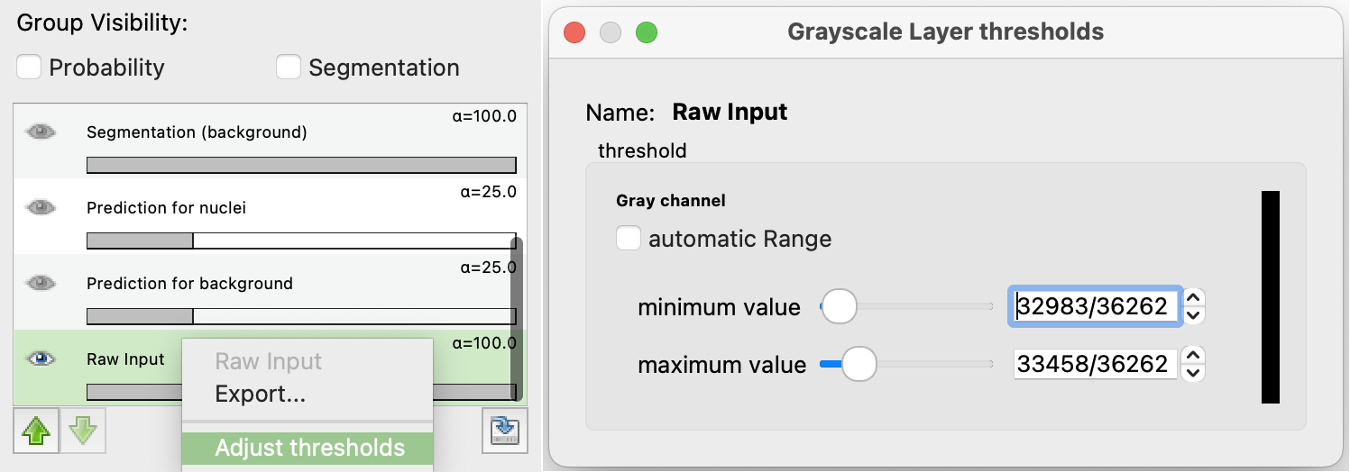
- To control brightness and contrast, right-click on Raw Input in the Group Visibility section (bottom left) and select Adjust thresholds to set the minimum and maximum display range.
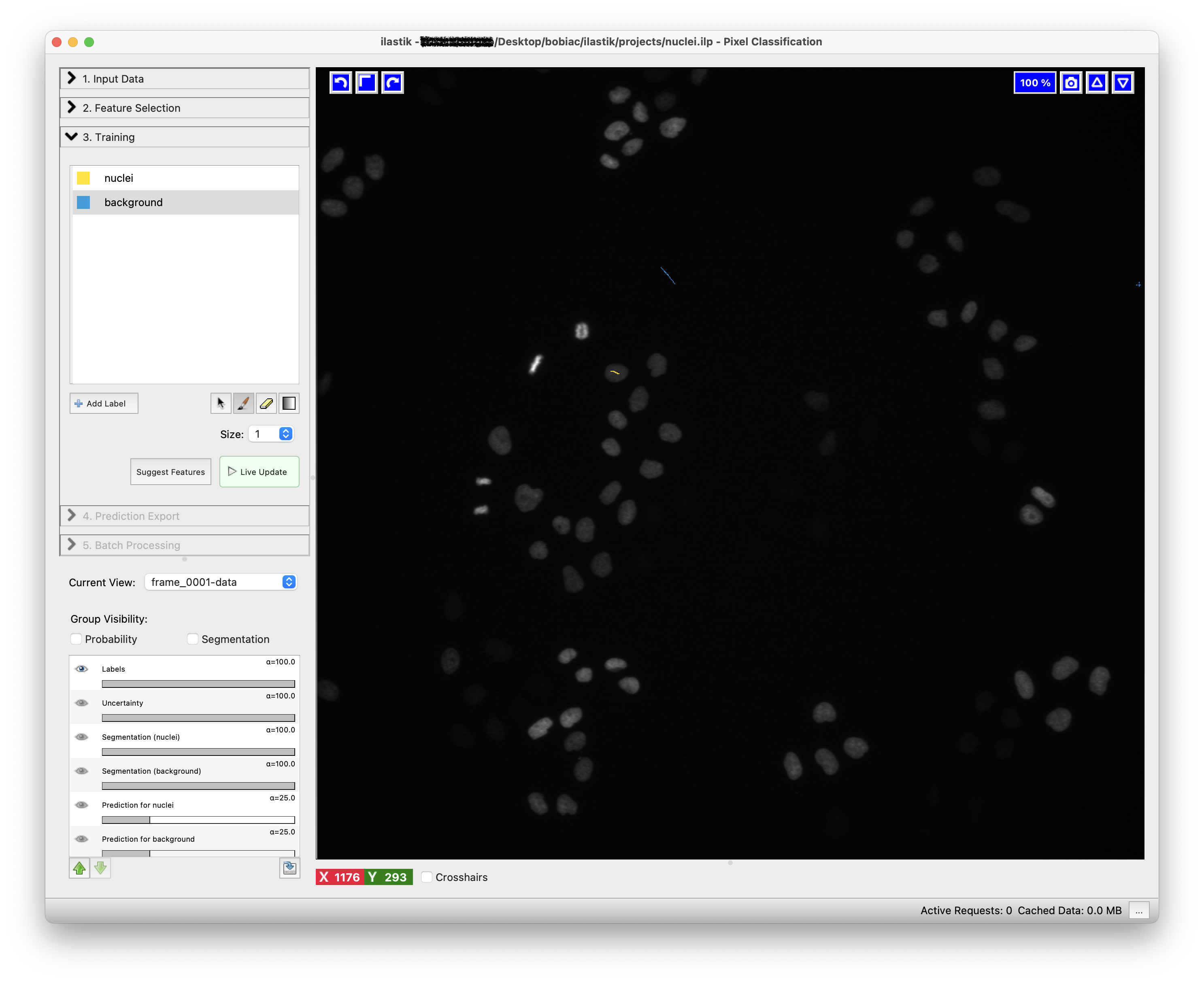
To train the classifier and see the predictions, press the Live Update button. This will update the predictions in real-time as you label more pixels.
The predictions will be displayed as an overlay on the image and colored according to the class colors you defined. Prediction overlay can be toggled on and off by pressing the p key on your keyboard.
In a similar way, you can visualize and toggle on and off the resulting semantic segmentation by pressing the s key on your keyboard.
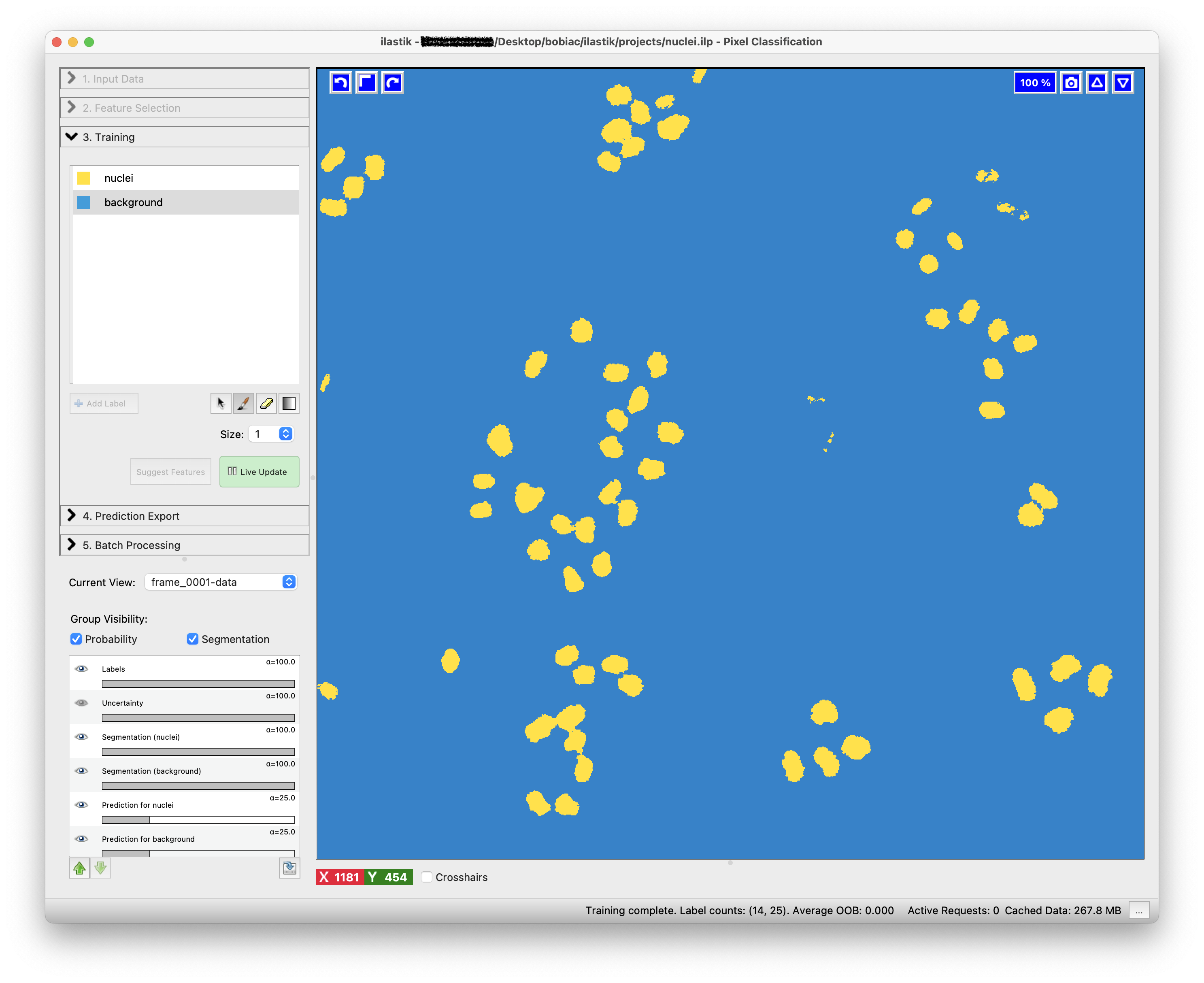
Examine the results for errors and add (or remove) annotations to correct.
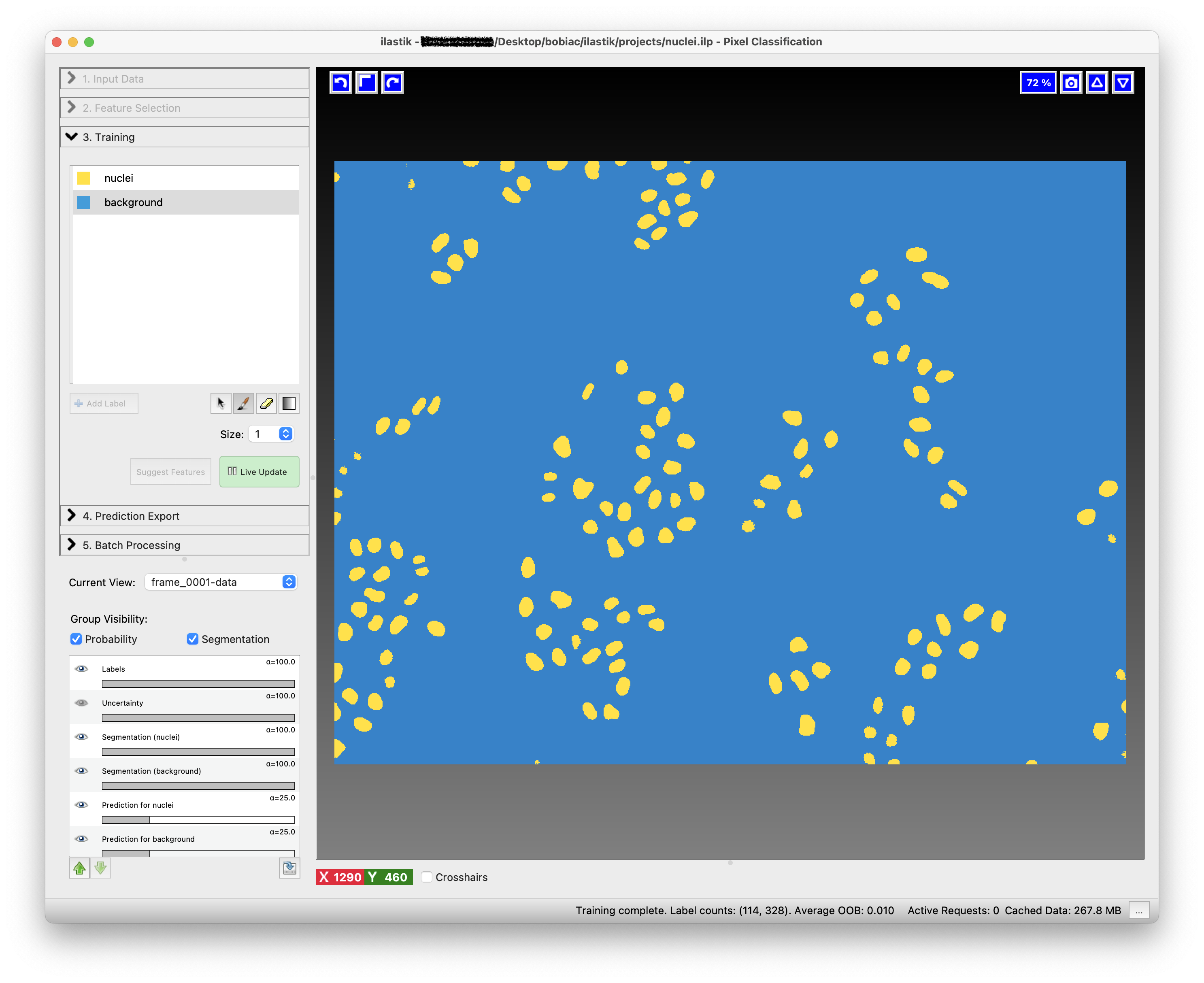
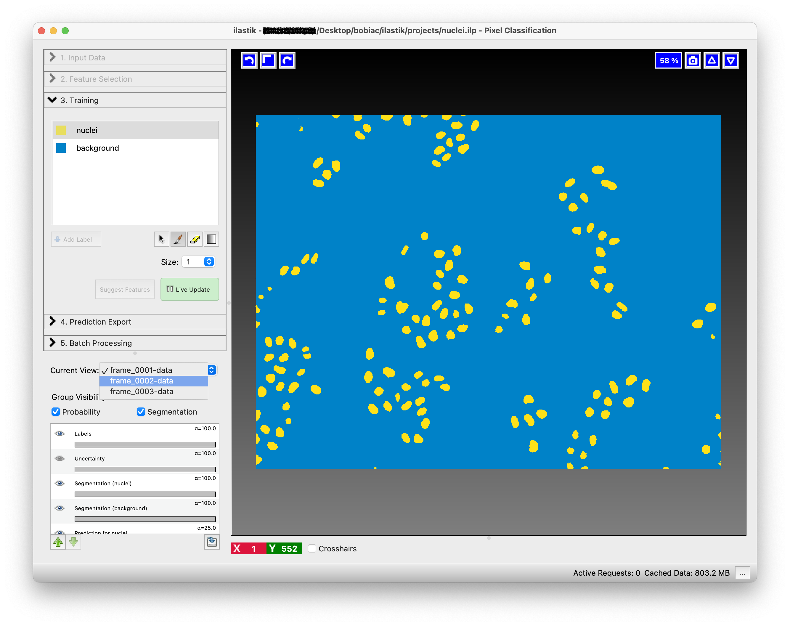
Once you are satisfied with the results, you now need to check if the classifier is robust enough to be applied to the rest of the images that you loaded at the beginning. To do this, you can switch to another image by clicking on the Current View drop-down menu on the left side of the GUI. Now activate again the Live Update to see the predictions for the new image. If the results are not satisfactory, you can keep Training the classifier add more annotations.
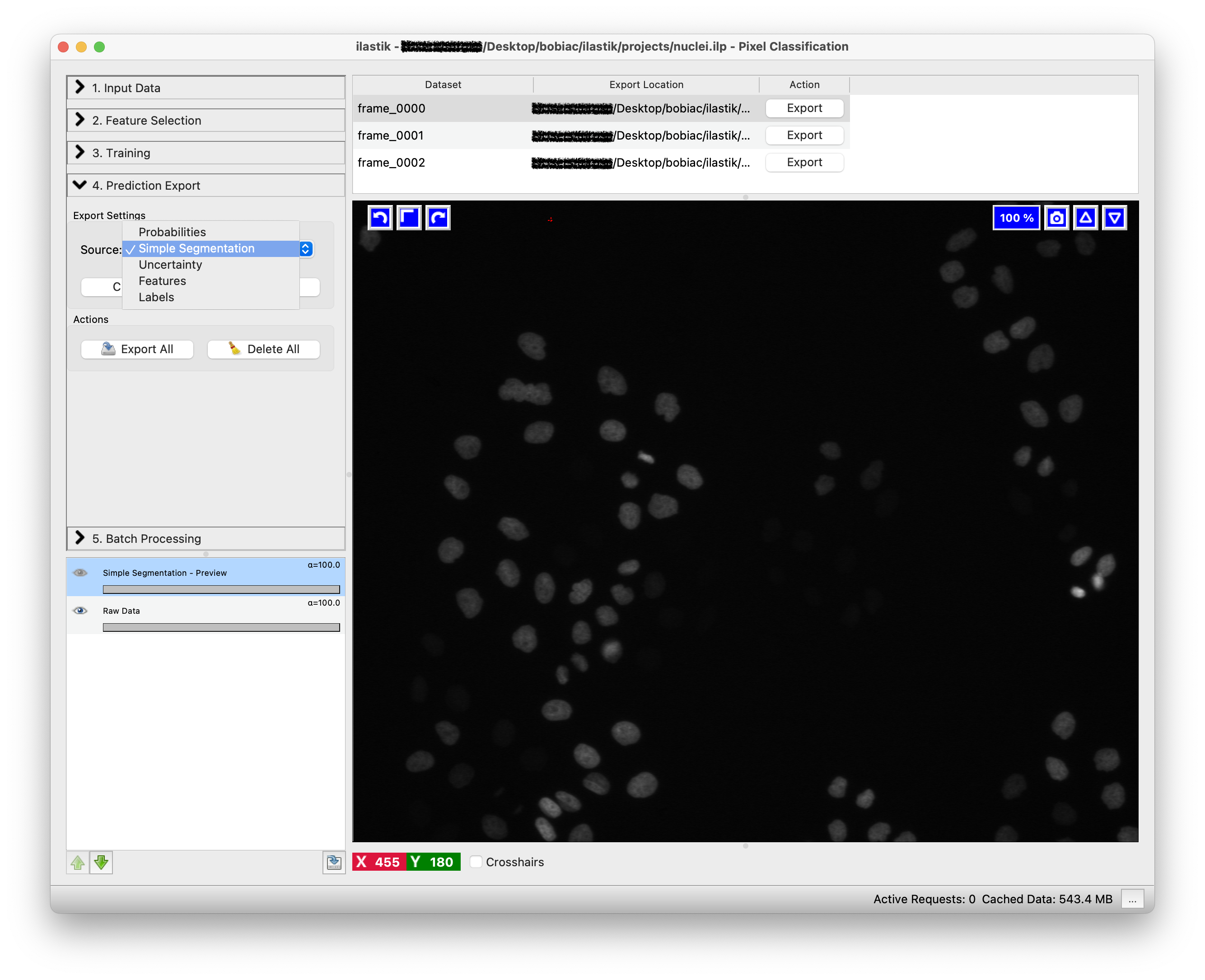
5. Export the Results#
Once the trained model works well with all the training images, you can either export the results (e.g. probability maps, semantic segmentation, …) for the training images or run the classifier in batch mode to process many images at once.
Either way, the first step is to select what you want to export by choosing an option in the Source drop-down menu in the Prediction Export step (on the left side of the GUI). Since in the next sections of the course we will use the semantic segmentation results, select Simple Segmentation. This option will export the semantic segmentation of the nuclei in the images, where each pixel is classified as either nuclei or background.
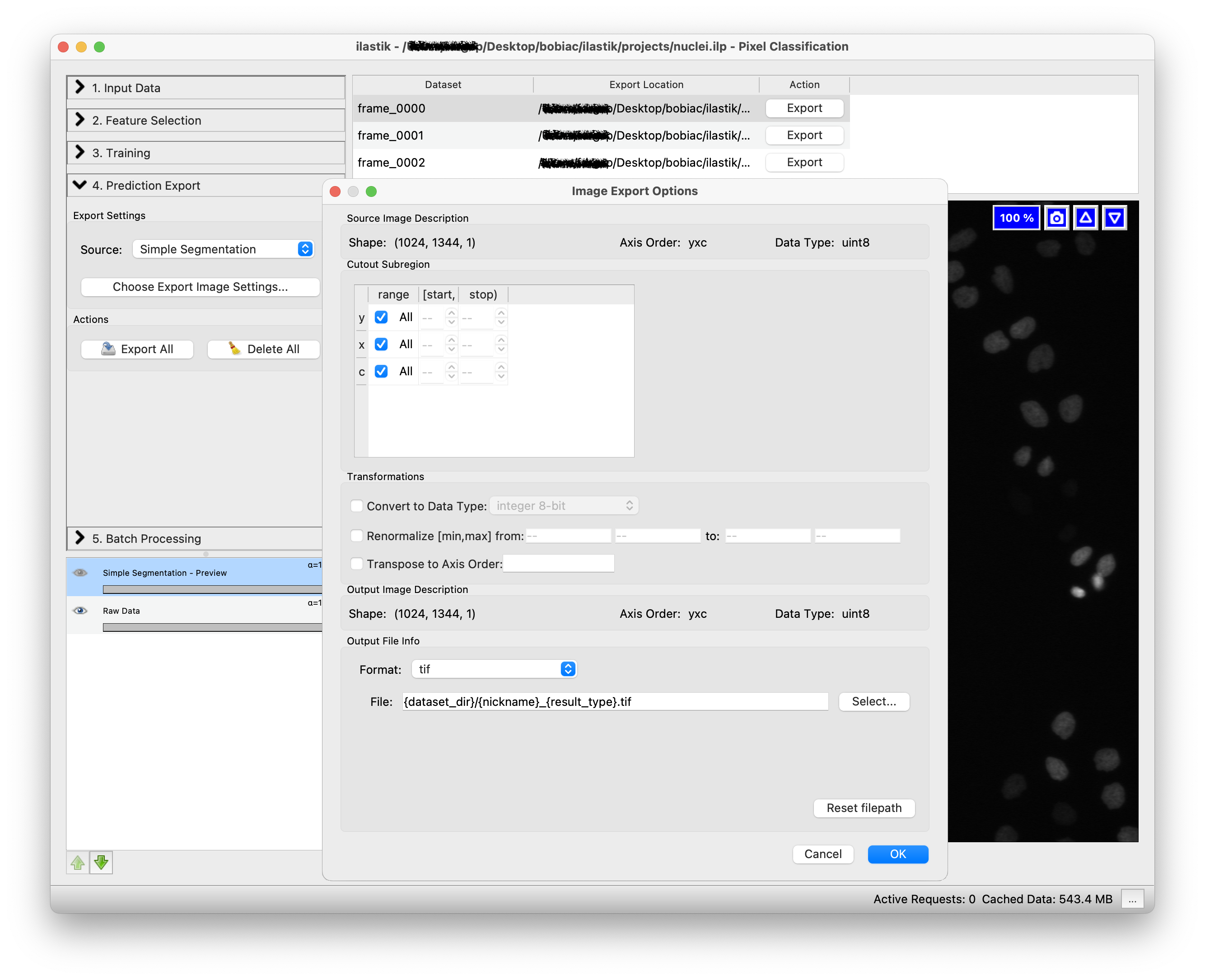
The second step is to select how we want to export the results. By clicking on the Choose Export Image Settings… button, a new window will open where you can select different options, including the export format and the output folder to save the result. Select “tif” as format and leave as default the output file path since it automatically is set to save the results in the same folder as the input images with the suffix appropriately changing depending on the option you select in the Source drop-down menu (e.g. _Simple Segmentation). Leave the other options untouched since we do not need to change them for this exercise.
Click on the Export All button to start exporting the predictions for all the training images. If you look in the folder where your training images are stored, you will find the exported results with the suffix _Simple Segmentation.

6. Batch Processing#
Since we will need to analyze more images for future sections of the course, we now want to run the classifier on all the images in the dataset. To do this, we need to select the Batch Processing step (on the left side of the GUI) and simply Drag and drop all the files in the dataset folder on the white area of the GUI.
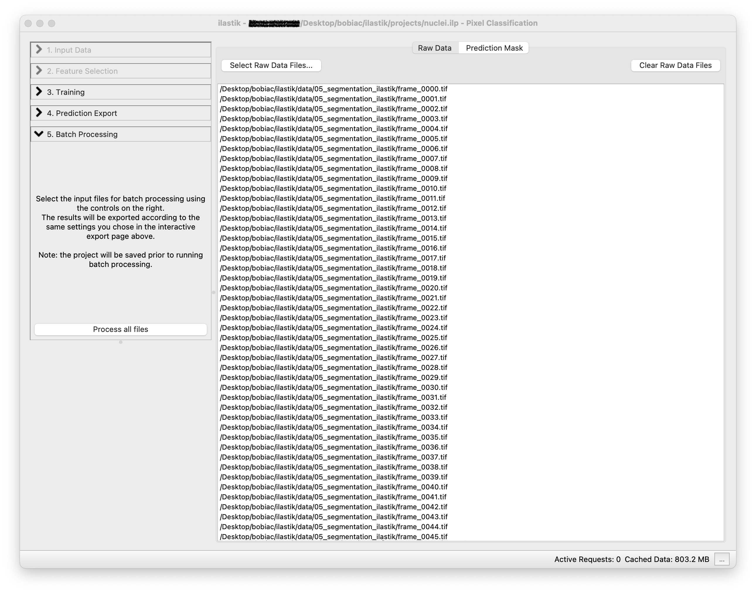
By clicking on the Process all files button, the classifier will be run on all the images in the dataset. Depending on the option you select in the previous Prediction Export, the results will be saved in the same folder as the input images with the corresponding suffix, in our case _Simple Segmentation.tif.
7. What’s Next?#
From this Ilastik pipeline we managed to extract the semantic segmentation of the nuclei in all the images. In the next section of this lesson, we will use the semantic segmentation and convert it into instance segmentation (as in the classic segmentation methods section. Then, we will classify nuclei in these labeled images into different cell cycle stage classes using the Ilastik Object Classification workflow.