# /// script
# requires-python = ">=3.11"
# ///
from pathlib import Path
from datetime import datetime
import numpy as np
from PIL import Image
import imageio
import skimage
import pooch

import matplotlib.pyplot as plt
%matplotlib inline

Intro to image segmentation – Global BioImaging Data Course - Pune, India

Student version:

Solution:

Welcome to the image segmentation chapter!
Just like the previous notebook, it is an interactive book: read, explore, and do.

You will learn core building blocks:

Chapter	Concept	Why it matters
0	What is image segmentation?	Semantics vs instance segmentation
1	Gaussian smoothing + Otsu threshold	Simple foreground / background separation
2	Watershed	Split touching objects into individual pieces

Each chapter follows the same pattern:

---

0. What is image segmentation?

Segmentation means labeling each pixel so that we can tell which pile of pixels belongs to which real‑world object.

There are two main types of segmentation:

• Semantic segmentation: Label each pixel with its class (e.g. "stroma", "cytoplasm", "background"). Good for tissues.
• Instance segmentation: Label each pixel with a unique ID for each object (e.g. "cell 1", "cell 2" or "nucleus 1", "nucleus 2"). Good for cell-based analysis.

In bioimage analysis that usually means turning a fluorescence snapshot into a binary mask of some cellular, subcellular, or tissue structure. Once you have a mask you can measure size, shape, intensity, count cells, follow them over time – all the good stuff.

There are many ways to segment.
Today we will cover two classical yet powerful techniques that get you surprisingly far:

Chapter	Technique	Typical use‑case
1	Gaussian + Otsu threshold	Simple foreground / background separation
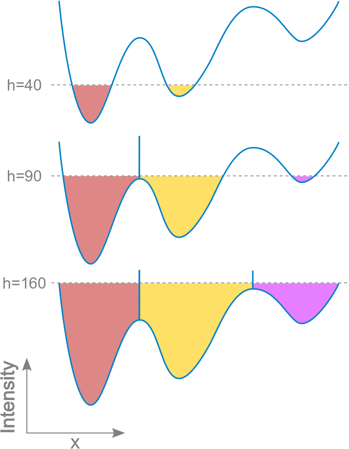
2	Watershed	Split touching objects into individual pieces

Each chapter follows the same pattern:

1. Theory – short, intuitive overview (no equations needed).
2. Live demo – run the code and poke at the parameters.
3. Your turn – exercises marked with ✍️ to make you write code.

Ready? Scroll on!

---

1. Gaussian smoothing + Otsu threshold

1.1 Intuition

Real microscope images are noisy.
Noisy pixels can trick a thresholding algorithm, and also sometimes we don't want to detect small details, so we smooth the image first with a Gaussian blur from skimage.filters.gaussian_filter:

clean = gaussian(image, sigma)

• sigma ≈ size of the noise blobs (in pixels).
• Big sigma ⟶ more blur, fewer details.

Then we separate foreground & background, first, using the simplest thresholding method.

Then, we can threshold in a more automatic way using Otsu’s method (skimage.filters.threshold_otsu).
Otsu finds the threshold that minimises the variance inside each class while maximising the variance between classes – no parameter to tune!

Finally we create a binary mask in a similar fashion:

mask = clean > thresh

That’s it – three lines for a first segmentation pass.

✍️ Exercise: your turn!

1. Re‑run the cell above with different sigma values (try 0.5, 1, 4, 8).
   How does blur influence the threshold and the mask?
2. 🏆 Challenge: compute the percentage of pixels classified as foreground for each sigma and plot sigma vs % foreground.

Extra point if you use a for loop!

Add extra cells below – the notebook is your sandbox!

Noticing all the little speckles in the mask? We can use morphological operations to clean it up:

1. Add a morphological opening (skimage.morphology.binary_opening) before remove_small_objects to get rid of speckles.
2. Add a morphological closing (skimage.morphology.binary_closing) after remove_small_objects to fill holes.

---

2. Watershed – separating touching objects

Intuition

Imagine the grayscale image as a topographic surface:

• Bright pixels are hills, dark pixels are valleys.
• We punch markers in the valleys we know belong to different objects.
• Then we flood the landscape – water rises simultaneously from every marker.
• Where waters meet we build a dam → that becomes the watershed line separating objects.

In practice we often:

1. Compute a distance transform of the binary mask (distance to nearest background pixel).
   Peaks of this map lie at object centres.
2. Find local maxima of the distance map as markers.
3. Run skimage.segmentation.watershed on the negative distance map so water flows from centres to edges.

✍️ Exercise: your turn!

1. Change the min_distance in peak_local_max.
   Smaller min_distance ⇒ more markers ⇒ over‑segmentation.
2. Use skimage.morphology.watershed on the gradient magnitude (e.g. Sobel filter) instead of the distance map.
   Compare results.
3. 🏆 Challenge: compute area distribution of segmented objects and plot a histogram. Mark the mean and median.

Extra cell slots below – go wild!

---

Where to go next?

• Machine‑learning‑based segmentation.